It only became widely accepted knowledge that all matter in the world is made up of tiny elementary particles in the early 19th century.
Let's look at the the picture below. What do you think this image is a model of?

Students will develop an understanding of how populations evolve by studying the case of pocket mice. Students will use computational models to understand the connection between natural selection, and speciation.
Unit co-designed by Sugat Dabholkar in consultation with teachers at Schurz High School
CODAP is a computational tool for data analysis and representation developed and built by The Concord Consortium at https://codap.concord.org/
The first four lessons are based on a Howard Hughes Medical Institute (HHMI) Biointeractive (https://www.hhmi.org/biointeractive/pocket-mouse-evolution)
Lesson 5 is based on the lesson Evolution in Action: The Galápagos Finches Authored by Paul Strode for Howard Hughes Medical Institute based on data collected by Peter and Rosemary Grant, Princeton University.
This work is supported by the National Science Foundation (grants CNS-1138461, CNS-1441041 and DRL-1020101) and the Spencer Foundation (grant 201600069). Any opinions, findings, conclusions, and/or recommendations are those of the investigators and do not necessarily reflect the views of the funding organizations.

This is an introductory lesson for using certain types of computational models designed using a software called NetLogo.
In this lesson, students will learn -
We will focus on four computational thinking practices: data practices, modeling and simulation practices, computational problem solving practices, and systems thinking practices.
Several lessons in this curriculum use computational models designed using a piece of software called NetLogo. In this lesson, we will try to understand what computational models are and how to use them.
This lesson specifically focuses on learning science with computational models of emergent natural phenomena. Emergent phenomena are ones in which simple interactions between agents and their environment result in complex patterns. For example, a flock of birds (see below).
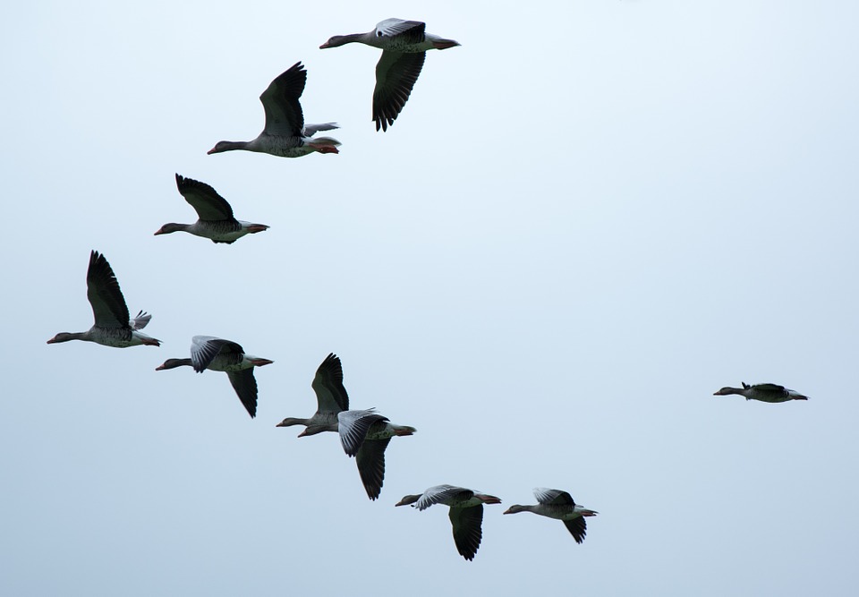
In a flock of birds, most people assume that the "head" bird is a leader of the flock. However, flocks actually emerge from each bird following a simple set of rules regarding how close and how far they should be from their neighbors as well as general direction of travel. This means that the shape of a flock is emergent and not directed by any particular leader bird.
We can use computational models to study and make predictions about emergent behaviors as long as we have a realistic understanding of the rules followed by the individual agents.
Learning Goals -
We will focus on four computational thinking practices: data practices, modeling and simulation practices, computational problem solving practices, and systems thinking practices.
Let's get started!
Scientists use scientific modeling approaches to construct knowledge about the world. In this section, we explore the ideas behind scientific models.
It only became widely accepted knowledge that all matter in the world is made up of tiny elementary particles in the early 19th century.
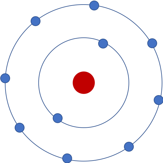
Let's look at the the picture below. What do you think this image is a model of?
Some of you probably said it's a model of an atom. Others might say it's a model of a 'Neon atom', because it has 10 electrons. In fact, since we don't know the number of protons, it could be an ion of a different element!
The point is that these representations in a model allow us to think about natural phenomena (like atoms containing electrons) that are associated with the model in certain way. Can you think of what this particular model could be useful for?
Now, let's look at a computational model of a forest. Imagine that you have a drone with a camera that is hovering above a forest. In other words, this model shows a top-down view of a forest. Each green patch you see represents a tree. A red patch represents a burning tree.
Play with the model and make some observations.
To run the model, make sure that you press 'setup' before you press 'go'.
What do you think a researcher or scientist could use this model for?
Make sure to change the density of trees in the model and observe the spread of the fire.
In this model, trees are called agents because their behaviors are programed into the model using a set of rules.
An example of one such rule is a tree cannot move. Another is when a tree is on fire it turns red. All trees follow the same set of rules.
How might you write a rule that a tree could follow that describes how they catch on fire?
Based on your exploration of the model, can you guess how the density of trees affects the spread of the fire in the forest?
This 'fire model' is a computational model, used to study how the interactions between the agents (trees) allows us to observe and understand emergent patterns like the spread of fire in the forest. Because it is a computational model, we can easily change parameters/variables such as the density of trees and then study how that change affects the spread of fire in the forest. Although this is just a model, we can use that knowledge to make predictions regarding the spread of fire in a real forest.
However, this model does not include all the factors that affect the spread of fire in a real forest. Brainstorm several other factors that might affect the spread of a real forest fire that could be added to this model?
Let's investigate how the density of the trees affects the spread of a forest fire. We will first generate some data using the Fire model and then visualize that data using another computational tool called CODAP.
Follow the experimental design that is described below:
Research Question: How does the density of trees in a forest affect the spread of a forest fire?
Hypothesis: As the density of trees in the forest increases, the percentage of forest burned will increase "linearly". (That means, if density of trees doubles, the percentage of forest burned will also double)
Let's test our hypothesis using the model.
Change the values of density systematically (plan out a series of different values to try). Record the value of 'percentage burned' in the data table for each density. Make sure that you press the 'setup' button every time you do a trial. Make sure to run each different value of density twice (2 trials) and finally, make sure you record values for each experimental trial.
CODAP will automatically graph the average of the two trials that you will record.
Write some observations about the graph of 'density%' vs 'percent burned average'.
Do you think that the evidence that we gathered with our experiment supports our hypothesis?
Explain your answer to the previous question.
The spread of a forest fire is an emergent phenomenon. Below a certain density, the fire does not spread much, however when the density crosses a 'tipping point' or threshold, the fire engulfs almost the whole forest.
The tipping point in this model falls within which of the following density ranges?
Can you give an example of another phenomenon with a tipping point?
This unit introduces computational thinking practices which include data practices, modeling and simulation practices, computational problem solving practices, and systems thinking practices. These practices are introduced to students in the context of a biology unit about ecology.
In this lesson, you will build and explore computational models of living systems. A special type of scientist called computational biologists, use computational models to study biological systems.
This unit focuses on prey-predator interactions in an ecosystem. It uses two computational modeling environments - NetTango and NetLogo.
NetTango is a block-based coding environment. It uses blocks to create a code for a computer program to perform certain tasks.
NetLogo is text-based coding environment. It uses text to write code for creating computational models.
As you spend your time learning about how to construct computational models of prey-predator ecosystems, you will learn a bit about coding using blocks as well as text.
Isle Royale
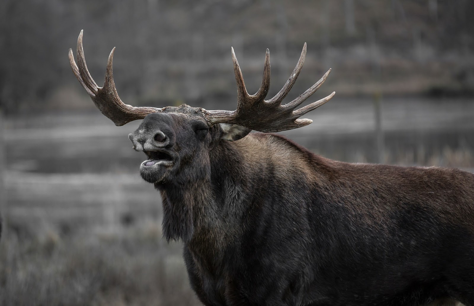
Ecosystems are often difficult to understand because they usually include interactions between a large number of species. Isle Royale is different. It is a relatively simple island ecosystem, located 24 km from the shore of Canada in Lake Superior.
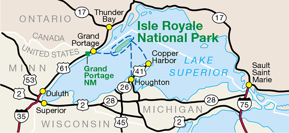

While there are many types of small animals on the island, and almost 20 types of mammals, only two species of the mammals that live on the island are relatively large. These are the wolves and the moose. On this island, wolves are the only predator of moose, and moose are essentially the only food for wolves.
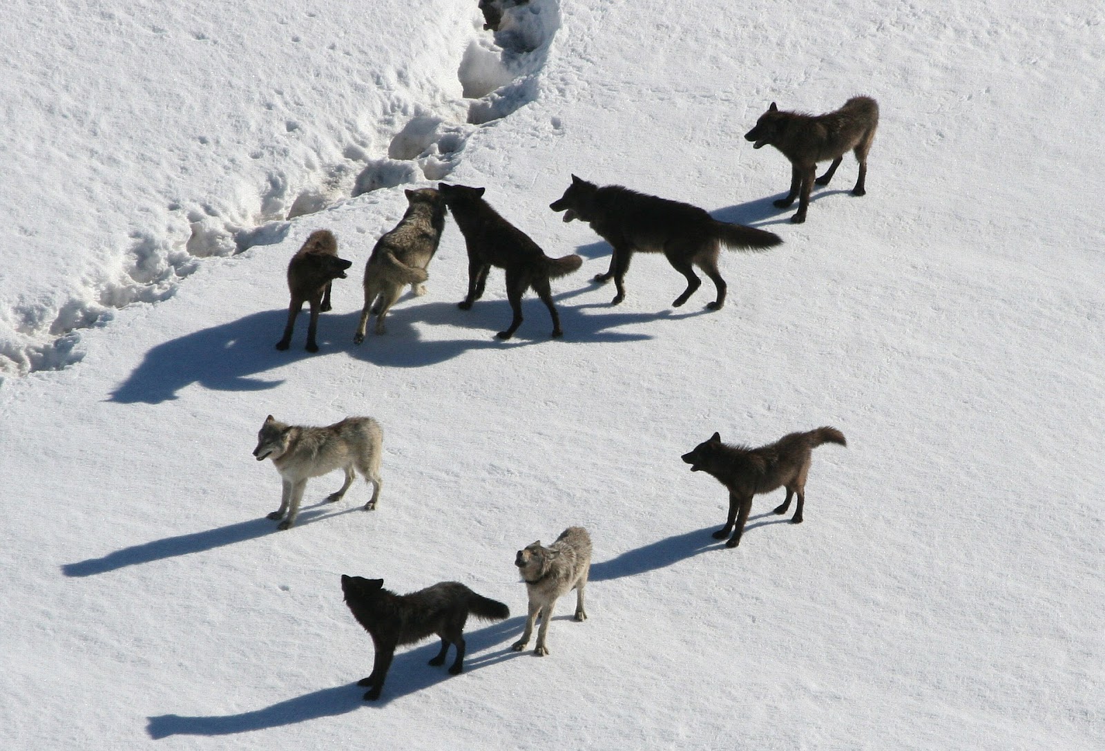
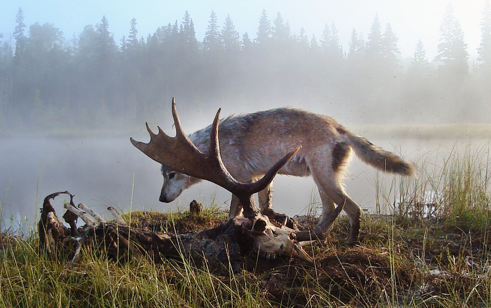
To understand nature, it helps to observe an ecosystem where human impact is limited. On Isle Royale, there are no towns and people do not hunt wolves or moose or cut down any of the forests. It is a very rare place on the planet where wolves, their prey, and the plants that support the prey are all left unharvested by humans. Isle Royale is remarkable because nature runs wild there.
Your challenge over the course of the next few days will be to build a scientific model that can realistically simulate the interactions of wolves and moose on Isle Royale, in order to help make predictions about how these two populations may change over time.
Thinking about this community of wolves and moose in Isle Royale, do you believe that the size of the wolf population will change from one day to the next?
Do you believe that the size of the wolf population will change from one month to the next?
Do you believe that the size of the wolf population will change over the course of 30 years?
Since wolves can’t typically migrate on or off the island, what other factors might cause the size of the wolf population to change from year to year?
Describe what may cause changes in the population of wolves and moose over time.
Let's start with building a simple model.
Try the following challenges:
Which blocks did you use to make the wolf move around the field? Choose all that apply.
Does the wolf look like it’s walking around the whole field or is it just going in a straight line or circles? If the moose aren't moving does the wolf get to all of them over time? Choose all that apply. Hint: Use the pen down block to have the wolf mark it's path.
After you have gotten your wolf moving, spend time trying to figure out the best block combination needed to get more realistic wolf movement. Try changing the numbers found in some of the blocks. What combination of blocks did you use to get realistic movement?
What blocks did you use to get the wolf to draw a dashed line?
If you could, what other types of behavior blocks would you add to make a more realistic wolf and moose predator/prey model?
The poor defenseless moose should be allowed to move as well! Start by setting up realistic movement for both wolves and moose and then move on from there.
Try the following challenges:
Which blocks did you use to make the wolf eat the moose? Choose all that apply.
Which blocks did you use to make the moose multiply? Choose all that apply.
Which block(s) did you use to slow down the moose reproduction?
What other behavior blocks could you add to this model to help make it more realistic?
Describe the challenge that you created and how you completed it.
Now that students have built a basic model, we're going to try and use this model to make predictions about the future of Isle Royale and the effects of different potential conservation efforts.
Now that we have a basic model, let's try to use it to predict what might happen in the future to Isle Royale.
Recently the Isle Royale ecosystem has been suffering. Since it has been isolated for a very long time, inbreeding has made the wolves less healthy. Also, there are very few wolves left on the island even though there are a lot of moose. We can use our model to try to predict what will happen in the future to Isle Royale.
In this lesson, you will use an advanced model of the ecosystem on Isle Royale to make a prediction.
First we need to set the model up so that it starts close to the current state of the island. There are very few wolves left and a lot of moose, so set the initial wolf population to 2 and set the initial moose population to about 200.
Because the wolves are unhealthy, decrease the WOLF-GAIN-FROM-FOOD slider from 20 to 13 and decrease the WOLF-REPRODUCE slider from 5% to 3%. These two "sliders" will help us model the fact that the wolves on Isle Royale are sick. They have a harder time staying healthy and a harder time having baby wolves.
Answer the first two questions below before running the model.
Why do you think there are so many moose in the ecosystem right now?
Before running the model, make a prediction. Do you think the wolf population will survive, or will it die out?
Run the model with the speed slider all the way to the right. The model will stop after 500 ticks have passed. When the model stops, use the table below to record whether there are still wolves alive or not. Repeat this process at least 5 times.
Look at the results of your experiment. Do you think the wolves on the real Isle Royale have a good chance of surviving into the future? Explain your answer.
Many scientists think that the wolf population on Isle Royale will probably die out in the near future. However, it may be possible to save them through some human intervention. We can use our model to test how good different interventions might be.
Answer the first two questions below before you start using the model.
What do you think we could do on Isle Royale to increase the chances that the wolves will survive?
How could you make the change you suggested actually happen in our model? For example, what parameters would you change? How would you change them?
Make the change or changes you suggested in the model and test how often the wolves survive. Fill out the table below just like before.
Do you think your intervention worked? Explain your answer.
Give an example of how a scientist might use a model to study ecosystems. Think of something specific a scientist might want to learn by using a model like this.
Models are useful tools for scientists, but no model can do everything. Why might it be hard to use a model like this to study ecosystems?
Describe one big idea you have learned from this lesson.

In this lesson, students will be introduced to the 'anchoring phenomenon' of rock pocket mice, specifically how the color of the fur coat changed because of the change in the environment where they live. Students will explore a computational model of a population of rock pocket mice and observe changes in the population over time.
This lesson is based on a curricular unit developed by HHMI (https://www.hhmi.org/biointeractive/making-fittest-natural-selection-and-adaptation).
In this lesson, you will study a phenomenon about a population of rock pocket mice. You will explore a computational model of a population these mice and observe changes in the population over time. By the end of the lesson, you'll be able to explain how the color of fur coat of mice changed over time and how it may have been affected by the change in their environment.
The American Southwest is a fantastic place to study rock pocket mice with different fur coat colors. Ancestral pocket mice had light-colored fur coats that blended in with the rocks and sandy soil that was prevalent in the region. This kept the mice hidden from their predators (mainly owls). Then, a series of volcanic eruptions spewed a river of black lava more than 40 miles long that wove right through the middle of pocket-mouse territory. Lava flows created huge patches of dark rock among the surrounding light-colored sand.
Today there are now two forms of pocket mice:
Researchers noticed that rock pocket mice with a dark fur coat were more common on the dark lava flows, whereas the mice with light colored fur coat were more common on the light-colored sand. How might this have happened?
In orer to investigate this mystery, we're going to investigate this case of pocket mice evolution using computational models.
Let's start by watching a video developed by HHMI Biointeractive about this phenomenon.
Name at least two things that you found interesting in the video.
Write down at least two questions that you would like to investigate about the pocket mice in the desert of New Mexico.
Below is a computational model of a population of pocket mice.
Each clock tick in the model is a mouse-generation and in each generation, male and female mice move around randomly, search for a partner, and reproduce if they find a partner. The fur-coat-color of the mice is a trait that is passed down from one generation to the next.
Play around with the model. It is totally okay if you don't understand everything mentioned in the model. Just explore the model for a few minutes and then try your best to answer the questions below.
There are two fur coat colors, light and dark. Which of these is a homozygous recessive condition?
Explain how you figured out the answer the the previous question.
There are two alleles "A" (dominant) and "a" (recessive). What would the phenotype be of the genotype "Aa"?
Explain how you arrived at the answer to the previous question.
Based on your investigation using this model, modify your questions that you wrote before. Specifically, you want to try to change your questions so that you could actually investigate them using a computational model like the one you explored in this lesson.
Explain how you might design some experiments using the model you explored earlier to answer your research questions.

In this lesson, students explore the computational model of a population pocket mice further. Specifically, they investigate how inheritance works in this model.
In this lesson, you will continue to explore our computational model of pocket mice further. Today, you'll be investigating the concept of inheritance of a trait across generation and how it affects evolution of a population in the model.
Remember that in this model, there are mice with two types of fur coat colors: light and dark. Observable characteristics (also called as traits) like fur color, eye color, or blood type are referred to as phenotypes. These phenotypes, including the color of fur coats is determined by the genes that a mouse has.
There are two kinds of genes in this models that affect the fur coat color of mice.
While answering the following questions, make sure that the "PREDATION?" box is unchecked.
Change the sliders under the "Initial Settings" in the model. Make sure every time you change the sliders that you press SETUP afterwards so that you can actually see the effects of your new settings. Try to change the settings such that all the mice have light-colored fur. Once you get all mice with light fur, describe the initial settings you used.
What will happen after lots of generations if the initial population of mice all have light-colored fur?
Run an experiment to prove or disprove your answer to the previous question and explain your observations.
What will happen after lots of generations if the initial population of mice all have dark-colored fur?
Run an experiment to prove or disprove your answer to the previous question and explain your observations.
In this model, "AA", "Aa", and "aa" are genotypes of mice. As we saw earlier, the fur coat color of a mouse is dependent on its genotype. Based on your investigations so far, can you say which of the three genotypes applies to each of our two fur-colors (light and dark)?
Explain how the value set by the 'chance-of-predation' slider affects the population size.
(Try setting at least five different values and observing how it affects the model before explaining the effects.)
Start a new experiment with a mixed population: some mice with dark fur and some mice with light fur.
Let the model run for at least 100 generations ("ticks"). Now change the background and let it run for 100 generations again.
Repeat the experiment a few times with different backgrounds.
What sorts of things did you observe in your experiments?
What might explain the observations that you wrote down in the previous question?

In this lesson, students investigate how natural selection affects the genetic constitution of a population over time. They design and perform an experiment about natural selection in the case of rock pocket mice using a computational model to test their hypotheses.
In this lesson, you will investigate how natural selection affects a population of mice over time. You will design and perform an experiment about natural selection in the case of rock pocket mice by using a computational model to test your hypothesis.
In the previous lesson, you experimented with the concept of predation. In other words, you investigated how the mice being eaten by predators affected the population of mice differently in different types of environments. In nature, some individuals with certain traits (like fur color) have better fitness to survive and create offspring that can inherit those traits. In the case of our models, mice with certain phenotypes might have a advantage over other mice in different environmental conditions. Traits that gives an advantage would get passed to the next generation. As these traits are passed from each generation to the next, this process causes populations to change over time. We call these sorts of changes in populations natural selection.
Come up with a question about natural selection in case of the pocket mice which can be answered using this model.
One example of a question that could be answered using the model: If we introduce a mutant (with a dark-fur-coat) in a population of mice with light-fur-coats that are living in a mixed background environment, how will to population change after 500 generations?
Based on your earlier exploration of the model, try to guess the answer to your question and state it in the form of a testable statement (hypothesis) - something that you can test using the model.
Design an experiment to test your hypothesis. Explain your design.
Collect data from the experiment in an excel or word file.
Describe your observations and explain whether those support your hypothesis or not.
Upload a Word, Excel or any other file here if you have used it record and analyze data. You can also just take a screenshot and upload that.
You can't upload Google Sheets or Docs Files. If you'd like to, make sure to Export them as a Word or Excel file first.
| File | Delete |
|---|---|
Explain the conclusion of your experiment.
Mention and describe a big idea that you learned in this lesson.