CT-STEM

Lesson 5. The Central Limit Theorem

Author(s): Jacob Mills

Subject: Mathematics

Time: 1 class period, 42 minutes

Level: High School AP Statistics

Version: v4

Overview

Students will explore the relationship between the shape of the population distribution, the sample size and the shape of the sampling distribution.

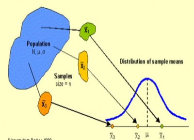
Central Limit Theorem demonstrates relations between population distributions and their sample mean distributions as well as the effect of sample size on this relation. In this model, a population is distributed by some variable, for instance by their total assets in thousands of dollars. The population is distributed randomly -- not necessarily 'normally' -- but sample means from this population nevertheless accumulate in a distribution that approaches a normal curve. The program allows for repeated sampling of individual specimens in the population

Standards

Computational Thinking in STEM 2.0

Computational Data Practices

[CT-DATA-1] Using computation to collect and create data
[CT-DATA-6] Using computation to analyze data

Computational Modeling and Simulation Practices

[CT-MODEL-1] Using computational models to understand a complex phenomenon
[CT-MODEL-2] Using computational models to hypothesize and test predictions

Activities

1. Exploring Central Limit Theorem in a NetLogo model
2. Exploring different population distributions
3. Reflection
4. Applications
5. Central Limit Theorem applications
6. Difference between Two Sample Means
7. Another difference of sample means problem
8. Some Final Thoughts

Student Directions and Resources

By the end of this lesson, you should be able to:

Explain how the shape of the sampling distribution of is affected by the shape of the population distribution and the sample size (aka, The Central Limit Theorem)
Explain why the Central Limit Theorem is one of the fundamental theorems in statistics
Calculate the mean and standard deviation of the sampling distribution of a sample mean \(\bar x\) and interpret the standard deviation
Calculate the mean and standard deviation of the sampling distribution of a difference in sample means \(\bar x_1- \bar x_2\) and interpret the standard deviation
Determine if the sampling distribution of \(\bar x_1- \bar x_2\) is approximately Normal
If appropriate, use a Normal distribution to calculate probabilities involving \(\bar x\) and \(\bar x_1- \bar x_2\)

1. Exploring Central Limit Theorem in a NetLogo model

Use the NetLogo model below to answer the questions.

Something has gone wrong. Please reload the page.

Question 1.1

In the NetLogo model above, press "SETUP" and then "Preset 1". Describe the shape of this distribution.

Question 1.2

Set the sample-size slider to 1. Try running the model by clicking the "go" button, which will run the model continuously until you click "go" again to stop. What do you notice about the shape of "Sample-Data Distribution"?

Question 1.3

If we ran the model for 100,000 or more samples (Preset 1, sample size = 1), what would the shape of the "Sample-Data-Distribution" be?

Question 1.4

Reset the model by clicking "setup" and "Preset 1". Set the "sample-size" slider to 5. Run the model by clicking "go" and note your observations below. How is this sample data distribution different from a sample size of 1?

Question 1.5

What's the takeaway? Explain the "big picture" idea of this page in a sentence of two.

2. Exploring different population distributions

Something has gone wrong. Please reload the page.

Question 2.1

Click "setup" and "Create My Own People" to create your own population distribution. Make sure your population size is greater than 50. Hint: instead of clicking once to create one person at a time, you can click and hold to create your population faster.

Need help? Watch this VIDEO

Question: How would you describe the shape of your population?

Question 2.2

Using the preset from your previous answer, start with a sample size of 10 and let the model run for at least 200 samples. Record the value of "std-dev-means" and the shape of the "sample-data-distribution".

Question 2.3

Reset the model and increase the sample size to 20. Run the model for at least 200 samples. What do you notice about the std-dev-means and the shape of the sample-data-distribution?

Question 2.4

Reset the model and increase the sample size to 40. Run the model for at least 200 samples. What do you notice about the std-dev-means and the shape of the sample-data-distribution?

Question 2.5

Compare the "std-dev-means" between a sample size of 10 and a sample size of 40. By what factor was the standard deviation reduced? (Hint: divide the two numbers to create a fraction)

Question 2.6

At a certain point, the sample-data-distribution becomes approximately Normal. What do you think is the cut-off for a sample size that produces an approximately Normal sampling distribution? Use the model above to answer this question.

3. Reflection

The Central Limit Theorem states that sample means from any population accumulate in a distribution that approaches a normal curve, as long as the sample size is "large enough". Our textbooks define "large enough" as \(n \ge 30\). This means that in order to produce a sampling distribution that is approximately Normal, we must sample at least 30 individuals from the population (if the population distribution shape is unknown or non-Normal). If the population distribution is Normal, the sampling distribution of \(\bar x\) will also be Normal, no matter what the sample size \(n\) is.

Question 3.1

Mr. Mills takes a sample of only 10 people and records their score on a particular IQ test. He is confident that he can make inferences about this sample using a Normal approximation. Why can he do this, even though his sample size was less than 30?

Question 3.2

In real life, we usually don't know what the population distribution looks like. Why can we make inferences about the population mean based on a large sample size?

Question 3.3

Explain how this physical model (see link below, called a Galton Board) can be used to describe the Central Limit Theorem. Click on link below to view a GIF of the Galton Board in action.

Galton Board

Question 3.4

Are there any other mathematical topics that you can think of when looking at the Galton Board?

4. Applications

From our formula sheet:

\(\mu_\bar X = \mu\) \(\sigma_\bar X = \frac {\sigma}{\sqrt n}\)

Trains carry iron ore from a mine in Brazil to an aluminum processing plant in Peru in hopper cars. Filling equipment is used to lode ore into the hopper cars. When functioning properly, the actual weights of ore loaded into each car by the filling equipment at the mine are approximately normally distributed with a mean of 70 tons and a standard deviation of 0.9 tons. If the mean is greater than 70 tons, the loading mechanism is overfilling.

Question 4.1

a) If the filling equipment is functioning properly, what is the probability that the weight of the ore in a randomly selected car will be 70.7 tons or more? Show your work.

Question 4.2

b) Suppose that the weight of ore in a randomly selected car is 70.7 tons. Would that fact make you suspect that the loading mechanism is overfilling cars? Justify your answer.

Question 4.3

c) If the filling equipment is functioning properly, what is the probability that a random sample of 10 cars will have a mean weight of 70.7 tons or more? Show your work.

Question 4.4

d) Based on your answer in part (c), if a random sample of 10 cars had a mean ore weight of 70.7 tons, would you suspect that the loading mechanism was overfilling the cars? Justify your answer.

5. Central Limit Theorem applications

Dr. Lopez gives students 90 minutes to complete the final exam for her course. Most students use almost all the time allowed, and relatively few students finish early, so the distribution of times that it takes students to finish the exam is strongly skewed to the left. The mean and standard deviation of the finishing times are 85 and 10 minutes, respectively.

Suppose we took random samples of 40 students and calculated \(\bar x\) as the sample mean finishing time. We can assume that the students in each sample are independent.

Question 5.1

What would be the shape of the sampling distribution of \(\bar x\)?

Question 5.2

Without doing any calculations, which of the following has a HIGHER probability:

1 randomly selected student taking more than 90 minutes to complete the final exam (meaning that they did not turn in the exam before the 90 minutes expired)
30 randomly selected students having a sample mean greater than 90 minutes

Justify your reasoning using appropriate statistical language.

Question 5.3

Explain why you cannot use a Normal distribution to calculate the probability of the first event in Question 5.2

6. Difference between Two Sample Means

From our formula sheet:

ACT scores at Ardrey Kell High School are Normally distributed with mean 26 and standard deviation 3. ACT scores at Providence HS are skewed to the right with mean 25 and standard deviation 5.

Question 6.1

We randomly select 25 students from AKHS and 30 students from PHS. Use the information given to describe the sampling distributions of the average ACT scores for the two samples.

Question 6.2

Suppose we took a sample of 25 students from AKHS and a sample of 30 students from PHS and found the difference in the sample means. Describe the sampling distribution of the difference in mean ACT scores (AKHS – PHS). Be sure to address shape, mean and standard deviation.

Question 6.3

Calculate the probability that random sample of 25 AKHS students has a higher mean ACT score than the random sample of 30 PHS students. Upload scanned image of work.

Upload files that are less than 5MB in size.

File	Delete

Upload files to the space allocated by your teacher.

7. Another difference of sample means problem

The heights of young men follow a Normal distribution with mean \(\mu_M\)= 69.3 inches and standard deviation \(\sigma_M \)= 2.8 inches. The heights of young women follow a Normal distribution with mean \(\mu_W\) = 64.5 inches and standard deviation \(\sigma_W\) = 2.5 inches. Suppose we select independent SRSs of 16 young men and 9 young women and calculate the sample mean heights \(\bar x_M\) and \(\bar x_W\).

Question 7.1

What is the shape of the sampling distribution of \(\bar x_M - \bar x_W\)? Why?

Question 7.2

Find the mean and standard deviation of the sampling distribution of \(\bar x_M - \bar x_W\)

Question 7.3

Calculate the probability that the average height of the 16 randomly selected men is less than the average height of the 9 randomly selected women.

Upload files that are less than 5MB in size.

File	Delete

Upload files to the space allocated by your teacher.

8. Some Final Thoughts

Please try to do your best to answer the following truthfully

Question 8.1

What is at least one big idea that you learned about sampling distributions in this unit? Explain.

Question 8.2

Pick any computational tool/activity that you have used in this lesson. Briefly describe the tool and explain how you used it to learn.