It only became widely accepted knowledge that all matter in the world is made up of tiny elementary particles in the early 19th century.
Let's look at the the picture below. What do you think this image is a model of?

Students will develop an understanding of how populations evolve by studying the case of pocket mice. Students will use computational models to explain the connection between genetic drift, natural selection, and speciation.
Unit co-designed by Sugat Dabholkar in consultation with Teresa Granito of Evanston Township High School
CODAP is a computational tool for data analysis and representation developed and built by The Concord Consortium at https://codap.concord.org/
The first four lessons are based on a Howard Hughes Medical Institute (HHMI) Biointeractive (https://www.hhmi.org/biointeractive/pocket-mouse-evolution)
Lesson 5 is based on the lesson Evolution in Action: The Galápagos Finches Authored by Paul Strode for Howard Hughes Medical Institute based on data collected by Peter and Rosemary Grant, Princeton University.
This work is supported by the National Science Foundation (grants CNS-1138461, CNS-1441041 and DRL-1020101) and the Spencer Foundation (grant 201600069). Any opinions, findings, conclusions, and/or recommendations are those of the investigators and do not necessarily reflect the views of the funding organizations.

This is an introductory lesson for using certain types of computational models designed using a software called NetLogo.
In this lesson, students will learn -
Several lessons in this curriculum use computational models designed using a piece of software called NetLogo. In this lesson, we will try to understand what these models are and how to use them.
This lesson specifically focuses on learning science with computational models of emergent natural phenomena. Emergent phenomena are ones in which simple interactions between agents and their environment result in complex patterns. Ffor example, a flock of birds (see below).
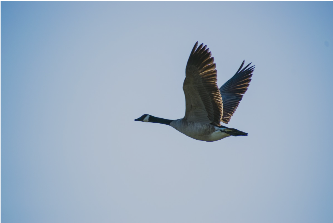
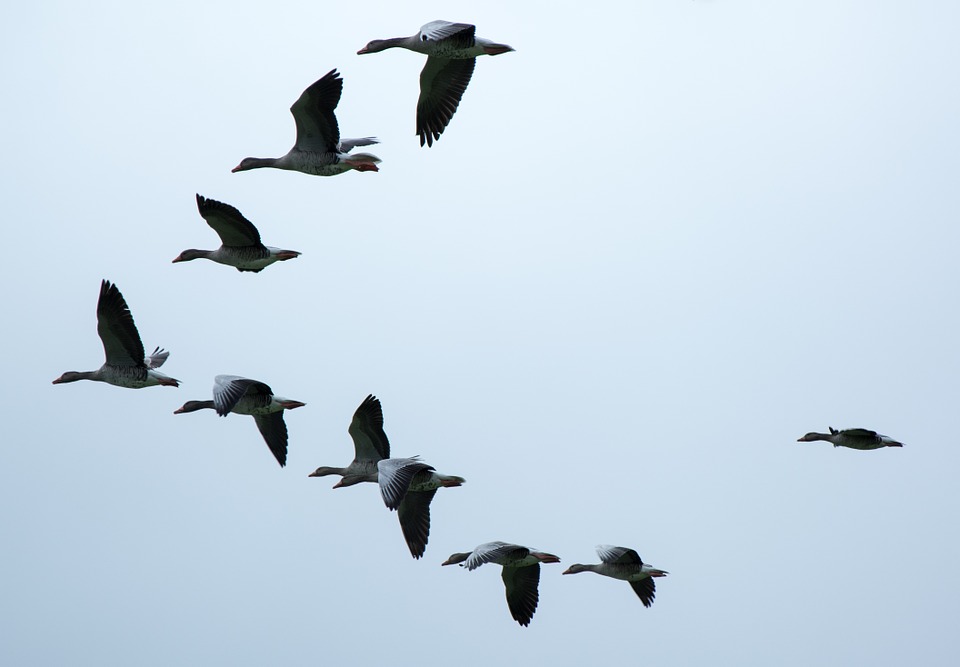
In a flock of birds, most people assume that the "head" bird is a leader of the flock. However, flocks actually emerge from each bird following a simple set of rules regarding alignment, coherence and separation with neighboring birds. This means that the shape of a flock is emergent and not directed by any particular leader bird.
Learning Goals -
Let's get started!
Scientists use scientific modeling approaches to construct knowledge about the world. In this section, we explore the ideas behind scientific models.
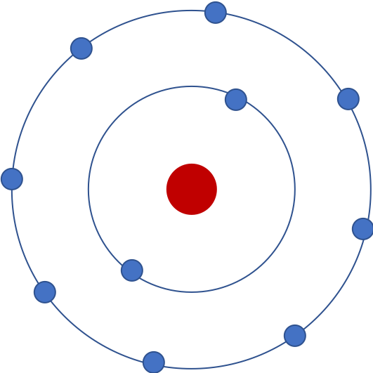
It only became widely accepted knowledge that all matter in the world is made up of tiny elementary particles in the early 19th century.
Let's look at the the picture below. What do you think this image is a model of?
Some of you probably said it's a model of an atom. Others might say it's a model of a 'Neon atom', because it has 10 electrons. In fact, since we don't know the number of protons, it could be an ion of a different element!
The point is that these representations in a model allow us to think about natural phenomena (like atoms containing electrons) that are associated with the model in certain way. Can you think of what this particular model could be useful for?
Now, let's look at a computational model of a forest. Imagine that you a drone with a camera that is hovering above a forest. In other words, this model shows a top-down view of a forest. Each green patch you see represents a tree. A red patch represents a burning tree.
Play with the model and make some observations.
What do you think a researcher or scientist could use this model for?
Make sure to change the density of trees in the model and observe the spread of the fire.
In this model, trees are called agents because their behaviors are programed into the model using a set of rules.
An example of one such rule is a tree cannot move. Another is when a tree is on fire it turns red.
How might you write a rule that a tree could follow that describes how they catch on fire?
Based on your exploration of the model, can you guess how the density of trees affects the spread of the fire in the forest?
This 'fire model' is an example of an emergent systems microworld. It is modeled in terms of interactions between the agents (trees) and it allows us to observe emergent patterns like the spread of fire in the forest. Because it is a computational model, we can easily change parameters such as the density of trees and then study how that change affects the spread of fire in the forest. Although this is just a model, we can use that knowledge to make predictions regarding the spread of fire in a real forest.
However, this model does not include all the factors that affect the spread of fire in a real forest. Can you suggest some other factors that might affect the spread of a real forest fire that could be added in this model?
Here's a version of a fire model that a team of researchers tried to modify, but it does not run as they expected. In fact, it's totally broken and does not run at all.
Can we help them fix it?
Setup the model. What is the mistake (or what you might hear people call a 'bug') in the researcher's model?
You probably noticed that after you press 'setup', you see blue colored trees. Maybe the bug in the code has something to do with the color of the trees. Maybe the color of the tree is set to 'blue' instead of 'green' by mistake.
Click on the bar that says 'NetLogo Code'. You can find it below the big square in the model.
Where does it say 'blue' in the code? And there does it say 'green' in the code?
You can fix that bug! Go to a line that say 'blue' where it should have been 'green'. Change the code.
Click on "Recompile code" and run the model again. Does it work now?
Can you explain why it did not work before?
These computational models, written in NetLogo, allow users to change the code and observe the effect of those changes. That is a very important feature of these Emergent Systems Microworlds: you can play with them and manipulate them by changing the parameters such as 'density' or by changing the code to see how the "microworld" you see is affected.
Now go back to the code and try to read some of it. The NetLogo language is designed to be easy to understand for humans. Pick a line in the code and paste it below. Try to explain how it affects the way the model would behave.
For example,
set initial-trees count patches with [pcolor = green]
This line sets a value for a variable 'initial-tree' by counting the patches that have pcolor (patch-color). This line is written in the NetLogo language that the NetLogo compiler understands.
Let's investigate how the density of the trees affects the spread of a forest fire.
We will first generate some data using the model and then visualize it using another computational tool called CODAP.
Let's follow an experimental design that is described below:
Research Question: How does density of trees in a forest affect spread of a forest fire?
Hypothesis: As the density of trees in the forest increases, the percentage of forest burned will increase linearly. (That means, if density of trees doubles, the percentage of forest burned will also double)
Let's test our hypothesis using the model.
Change the values of density systematically. Record the value of 'percentage forest burned' in the data table. Make sure that you press 'setup' button every time you do a trial. Make sure to run each different value of density twice and finally, make sure you record values for each experimental trial.
CODAP will automatically plot the average of the two values that you will record.
Write some observations about the graph of 'density' vs 'percentage burned'.
Do you think that the evidence that we gathered with our experiment supports our hypothesis?
Explain your answer to the previous question.
Spread of a forest fire is an emergent phenomenon. Below a certain density, the fire does not spread much, however when the density crosses a 'tipping point' or threshold, the fire engulfs almost all the forest.
The tipping point in this model falls within which of the following density ranges?
Can you give an example of another such phenomenon with a tipping point?
Explore a more detailed version of the fire model above.
Explain what "probability-of-spread" might mean in the model and how it would affect the behavior of the model.
Write a question that is of an interest to you which can be answered using this model.
An example of such a question would be: how does wind speed affect spread of fire?
Based on your exploration of the model, make a guess and state it in the form of a testable statement (a hypothesis)–one that you can test using the model.
Design an experiment to test your hypothesis. Explain your design.
Perform the experiment. Describe your observations and explain whether those support your hypothesis or not.

In this lesson, students will be introduced to the 'anchoring phenomenon' of rock pocket mice, specifically how the color of the fur coat changed because of the change in the environment where the live. They will explore a computational model of a population of rock pocket mice and observe changes in the population over time.
This lesson is based on a curricular unit developed by HHMI (https://www.hhmi.org/biointeractive/making-fittest-natural-selection-and-adaptation).
In this lesson, you will study a phenomenon about a population of rock pocket mice. You will explore a computational model of a population of rock pocket mice and observe changes in the population over time. You will be able to explain how the color of fur coat of mice changed because of a change in the environment where they lived.
The American Southwest is a fantastic place to study rock pocket mice with different fur coat colors. Ancestral pocket mice had light-colored fur coats that blended in with the rocks and sandy soil that was prevalent in the region. This kept the mice hidden from their predators (mainly owls). Then, a series of volcanic eruptions spewed a river of black lava more than 40 miles long that wove right through the middle of pocket-mouse territory. Lava flows created huge patches of dark rock among the surrounding light-colored sand.
Today there are now two forms of pocket mice:
Researchers noticed that rock pocket mice with a dark fur coat were more common on the dark lava flows, whereas the mice with light colored fur coat were more common on the light-colored sand. How might this have happened?
In the next few lessons we will investigate this case of pocket mice evolution using computational models.
Let's start by watching a video developed by HHMI Biointeractive about this phenomenon.
Mention at least two things that you found interesting in the video.
Mention at least two questions that you would like to investigate about the pocket mice in the desert of New Mexico.
Here is a computational model of a population of pocket mice.
The rules of interactions between the pocket mice are similar to the Hardy-Weinberg activity that you must have already done in class.
Each clock tick in the model is a mouse-generation. In each generation, male and female mice move around randomly, search for a partner, and reproduce if they find a partner. The heritable trait that is modeled here is fur-coat-color of the mice.
Explore the model and answer the questions below.
There are two fur coat colors, light and dark. Which of these is a homozygous recessive condition?
Explain how you figured out the answer the the previous question.
There are two alleles A (dominant) and a (recessive). What would the phenotype be of the genotype 'Aa'?
Explain how you arrived at the answer to the previous question.
Let's investigate how genotype frequencies change over time in this population.
The five conditions for Hardy-Weinberg law of genetic equilibrium are:
1. The breeding population is large.
2. Mating is random.
3. There is no mutation of the alleles.
4. No differential migration occurs.
5. There is no selection.
Do you think all the conditions of Hardy-Weinberg law of genetic equilibrium are satisfied in this model? Explain your answer.
Set the initial population such that it is not at Hardy-Weinberg genetic equilibrium. Write down your initial settings.
Write your initial allele frequency and phenotype frequency values.
Run your model for 15 generations (ticks). Note the Hardy-Weinberg equation values and genotype frequency values in the table below,
Explain your observations.
Based on your investigation using this model, modify your research questions that you wrote before.
Make the modifications such that you could investigate the new questions using a computational model such as the one you explored in this lesson.

In this lesson students will understand the basic idea of Hardy Weinberg Equilibrium. They will also calculate phenotype frequencies both mathematically and computationally (using a computational model).
In this lesson you will learn the basic idea of a Hardy Weinberg Equilibrium. You will also calculate phenotype frequencies both mathematically and computationally (using a computational model).
This model is same as the one that you used in the previous lesson. Just play with the model for a few minutes. Change the parameters and make observations.
If I am a mouse with dark fur color, what would be my genotype?
How would you test your answer to the previous question using the model?
Based on your initial exploration of the model, write down two observations that you find interesting.
A group of field researchers have estimated the frequency (p) of allele A as 0.7 and the frequency (q) of allele a as 0.3. Set the initial population in the model such that you get those frequencies. Make sure that the total population is greater than 200.
Write down the values you set for the following parameters below:
Also, write down the values for the Hardy-Weinberg equation values and genotype frequency values in the table below:
Run your model for 15 generations (ticks). Note the Hardy-Weinberg equation values and genotype frequency values again.
Discuss with your partner and others in the class and describe your observations.
Explain the observations that you mentioned as your answer to the previous question.
Write a question about the Hardy-Weinberg Law of Genetic Equilibrium that can be answered using this model.
An example of such question would be, how does the population size affect how fast a Hardy-Weinberg Genetic Equilibrium is reached?
Based on your exploration of the model, guess an answer to your question and state it in the form of a testable statement (hypothesis) - something that you can test using the model.
Design an experiment to test your hypothesis. Explain your design.
Perform the experiment. Describe your observations and explain whether those support your hypothesis or not.
* You can record your data in a word or excel file and upload it in the next question to support your answer.
Upload a word, excel or any other file here if you have used it record and analyze data.
| File | Delete |
|---|---|
Mention and describe a big idea that you learned in this lesson.

In this lesson, students investigate how natural selection affects the genetic constitution of a population over time. They design and perform an experiment about natural selection in the case of rock pocket mice using a computational model to test their hypotheses.
In this lesson, you will investigate how natural selection affects the genetic constitution of a population over time. You will design and perform an experiment about natural selection in the case of rock pocket mice using a computational model to test your hypothesis.
This model is similar to the previous model. Just play with the model for a few minutes. Change the parameters and make observations.
Write down at least three differences that you observe in this model as compared with the previous model.
Write down at least two observations that you find interesting in this model.
Explain how the value set by the 'predation' slider affects the population size.
(Try setting at least five different values before explaining the effects.)
Start with a mixed population. Let the simulation run for at least 100 generations. Now change the background. Let it run for 100 generations again.
Repeat the experiment a few times with different backgrounds.
Write down your observations.
Explain the observations that you wrote as your answer to the previous question.
Write a question about Natural Selection in case of the pocket mice which can be answered using this model.
An example of such a question would be: how does the genotype frequency of the population change if a mutant is introduced to a population of homozygous-recessive mice?
Based on your exploration of the model, guess an answer to your question and state it in the form of a testable statement (hypothesis) - something that you can test using the model.
Design an experiment to test your hypothesis. Explain your design.
Perform the experiment. Describe your observations and explain whether those support your hypothesis or not.
* You can record your data in a word or excel file and upload in the next question to support you answer.
Upload a word, excel or any other file here if you have used it record and analyze data.
| File | Delete |
|---|---|
Mention and describe a big idea that you learned in this lesson.

In this lesson, students investigate how genetic drift affects the genetic constitution of a population over time.
In this lesson, you will investigate how genetic drift affects the genetic constitution of a population over time. You will design and perform an experiment about genetic drift using a computational model to test your hypothesis.
You have already used this model. Answer the questions below to refresh your memory.
If you set the values of homozygous-dominant-males to 100 and homozygous-recessive-females to 100, and all the other values of initial males and females zero, what would be the values of p and q?
If you set the values of initial males and females as follows:
What would be values of p and q?
What about the frequencies of AA, Aa and aa?
Do you think the model, in its current state, satisfies all the Hardy-Weinberg Law of Genetic Equilibrium conditions?
Run the model for 15 generations with the conditions in the previous two questions. Note your observations.
Do you think that the Hardy-Weinberg law holds?
Explain your answer to the previous question.
Set the total initial population to less than 80. Make sure that it is a mixed population and there is at least one member of each genotype and gender. Run the model for at least 500 generations. Note your observations.
Repeat the experiment that you did for the previous question at least 10 times. Note down your observations.
Describe any patterns that you might have observed in the data you collected.
Why do you think the patterns observed above are happening? Explain your answer.
Write a question about genetic drift in the pocket mice population which can be answered using this model.
An example of such question would be, 'how does population size affect the extinction of an allele from the population?' or 'is it more or less likely for a recessive allele to go extinct as compared with a dominant allele?'
Based on your exploration of the model, guess an answer to your question and state it in the form of a testable statement (hypothesis) - something that you can test using the model.
Design an experiment to test your hypothesis. Explain your design.
Perform the experiment. Describe your observations and explain whether those support your hypothesis or not.
* You can record your data in a word or excel file and upload it in the next question to support you answer.
Upload a word, excel or any other file here if you have used it record and analyze data.
| File | Delete |
|---|---|
Mention and describe a big idea that you learned in this lesson.

CODAP is developed and built by The Concord Consortium at https://codap.concord.org/
This lesson is based on the lesson Evolution in Action: The Galápagos Finches Authored by Paul Strode for Howard Hughes Medical Institute based on data collected by Peter and Rosemary Grant, Princeton University.
It uses an HHMI video: https://www.youtube.com/watch?v=mcM23M-CCog
The purpose of this lesson is to learn how the combination of mutations, natural selection, and environmental change generate progressively better-suited adaptations.
Purpose
So far we have studied how environmental changes affect population of species. In this lesson, we will explore how new species emerge.
Brainstorm
You know that many species that were alive in the past have gone extinct. Many of the species that are alive today did not exist at one point in the past.

Explain how natural selection could help to explain how new species might emerge. Think back to some of the earlier concepts you went over.
Can evolution occur without natural selection?
There are 13 species of finch on the islands, but they are at once both so similar and so diverse that they have provided a fertile ground for exploring evolution since Darwin’s 1835 visit. Darwin himself did not realize their role in explaining evolution until after ornithologists revealed the abundance of speciation to him.
Let's watch a video developed by Howard Hughes Medical Institute based on data collected by Peter and Rosemary Grant, Princeton University.
The finches are proposed to have arrived on the volcanic islands from the South American mainland and are now considered part of the tanager family rather than the finch family. There are four genera recognized in the group, and the species occupy overlapping but distinct ecological niches. In the genus Geospiza, there are six species. In good times, they often eat the same foods, but in times of scarcity, each species has a specialized niche – large seeds, cactus fruits, etc. – on which they rely. Their mating behaviors, such as times and songs, differ greatly, maintaining the distinct species. The ecology of the different islands influences which species live on each island, and especially which species co-exist on an island. Gene flow between islands occurs with occasional immigrants depending on storms and the distance between islands.
For several decades, scientists have gone to the Galapagos islands to study the physical characteristics of the finches there. They recorded data on many traits including beak dimensions and weight. In this lesson you will explore some of that data to understand the processes underlying speciation and adaptive radiation.


What do you think separates species from each other? In other words, what does it mean to be a 'different species' than another organism?
How would you go about trying to distinguish one species from another?
Why do you think the data the scientists collected might be useful for studying differences between species?
Below is a data analysis tool called CODAP created by educators at the Concord Consortium. Using this computational tool, you will be able to delve deeply into the finch data mentioned on the previous page. When the page loads you will see the basic finch dataset with columns for sex, weight (g), beak length (mm), beak depth (mm). In CODAP we are able to interact dynamically with the data, allowing us to make connections and draw conclusions. We will use this set to answer several questions about these Galapagos finches.
Use CODAP to fill out the following data table.
You can see the value of a data point by hovering your mouse over the point. Use this to find the minimum and maximum beak lengths.
Clicking on the data point will highlight the row in the data table.
Clicking on a graph will cause a toolbar to appear next to it. You can find and display useful information about the data in a graph using the ruler menu in that toolbar. Click the check boxes for median, mean, and standard deviation to display them on the graph. You can find their values by hovering your mouse over the display.
If you click and drag to surround points on a graph, they will be selected on all current graphs. You can use this to hide points that you don't want to see. Sometimes CODAP responds slowly and will have a slight delay, so you may need to wait for it to catch up.
Click and drag to select all of the male finches. Then, on the histogram of beak length, use the eye menu to the right of the graph to hide unselected points. For clarity, you can also change the title of the graph to "Males" by clicking on the current title in the blue bar at the top of the graph.
What is the mean beak length for male finches?
In order to visually compare two or more subgroups, it can be helpful to have multiple graphs. Sometimes the points on a new graph will not look the same as those on other graphs. You can change the appearance of the points on any graph using the paintbrush menu to the right of the graph.
In the upper left corner, click the "Graph" button to create a new blank graph. Drag the "Weight" column header from the table to the x-axis of the new graph to create a second histogram and title it "Females". Using the same method as before, hide all of the points on the new plot that aren't from female finches. Drag the "Weight" column header to the x-axis of the original graph to replace "Beak Length".
What differences do you notice in the graph of male finches vs. the graph of female finches? Be sure to mention characteristics like shape of the graph and median values.
Another way to compare subgroups is to put categorical data on the y-axis. Close one of the two histograms and use the eye menu to show all points on the remaining graph. If you want, you can change the title for clarity. Then, drag the "Sex" column header to the y-axis of the histogram.
How does the group of finches of unknown sex compare to the male and female finches?
Drag the "Beak Length" column header to the y-axis of the histogram to turn it into a scatter plot. If you still want an idea of how the male, female, and unknown sex finches compare, you can drag the "Sex" column header to the middle of the plot to change the color of each point to match the sex of the finch.
Based on this plot, what seems to be the relationship between weight and beak length in these finches?
The data above comes from only one species of finch. Why do you think there is variation in the beak lengths and weights of these finches? Think back to some of the earlier lessons when you saw a graph like this.
The scientist that have collected this data have done so for over 40 years now, the first bar graph that you saw in section one contains finch data from 1973 -1981. Lets see what we can find if we look deeper into the data.
In this data set, "Last Year" is the record of the last year an individual finch was seen by the researchers. This typically means that the individual finch died during that year.
Use the methods you learned in the last activity to compare the finches that died during 1977 with the finches that survived 1977 and answer the questions below.
What differences do you see between the group of finches that only lived until 1977 and the finches that lived to 1978 and beyond? Please discuss the position (i.e. mean, median) and shape (i.e. standard deviation, range) of the beak depth distributions in your response, along with any other information you think is relevant.
|
The medium ground finch (Geospiza fortis) has a short, blunt beak which is adapted to picking up seeds from the ground. In 1976, seeds on the island were diverse and plentiful. During a drought in 1977, seeds became much harder to find. Once the finches had eaten all the small and medium-sized seeds, they had to turn to larger, spiny seeds that are hard to crack open. In your group come up with a reasonable hypothesis as to why there might be changes in how beak depths are distributed before and after 1977. Think about connecting past ideas like competition and natural selection. Be as specific as you can. |
|
| During the drought, the beak depth with the greatest fitness increased, but the amount of variation in the trait did not. This is an example of directional selection. Directional selection is often the result of a change in environmental conditions. How does this compare to the stabilizing selection you saw in the previous lesson? |  |
This CODAP frame has a much larger data set than those you have explored in the previous activities. To help you gain a better understanding of the finches in the Galapagos, there are many more physical traits to explore. Use the skills you developed in the previous activities to use CODAP to look at several traits and compare them across species and locations.
Not all of the traits were measured on each individual, so some traits will have more complete information than others. We will focus on a trait that has a lot of data points, beak height.
Generally speaking, how are the different finch species similar or different?
For example, which species have similar ranges of beak height? Which species have different ranges of beak height?
Generally speaking, how are the finches on different islands similar or different?
For example, you might think about whether the islands all have the same species, or whether the islands all have similar distributions of beak height.
Generally speaking, are members of the same species on different islands different from each other? Give examples to support your answer.
Look at the histogram of beak heights for all finches. There appear to be several peaks in it. Are there multiple species or islands represented in each peak? What does this suggest about the niches present in this ecosystem and the species that are in a peak together?
Do the answers to any of these questions change if you look at another trait with many data points, like wing length or N-UBkL (another measure of upper beak length)? How?


Scientists think the finches on the Galapagos are descended from finches that traveled from the mainland at some time in the past. One possibility is that one type of finch arrived at the islands and split into new species over time. Another possibility is that several species arrived at the islands. Which do you think is more likely? Why?
Do you think the environments on each island are similar? How might they be different? It may be helpful to think about this in terms of ecological niches, and to think back to what you saw in the previous activity.
Why do you think there are so many different species of finch on such a small group of islands? How might differences between the islands and their niches have affected the number of species?
Come up with a story that describes the how the different species of finches could have developed in the Galapagos islands.

Purpose: The purpose of this activity is to understand how new species can form from old species through the mechanisms of evolution covered so far in the unit (mutation, genetic drift, changes in environmental conditions, and natural selection).
Connection to previous activities: Students refer to the mechanisms of mutation (introduced in the last activity), genetic drift (from the activity before that), changes in environmental conditions and natural selection (from two previous activities), to develop the explanations for the outcomes in this activity.
Learning Performances
• Analyze data from a computer investigation applying concepts of statistics and probability to explain why adaptations for reproductive isolation can help reinforce specialized adaptations for survival for different niches within different gene pools in a population. [Emphasis is on analyzing shifts in numerical distribution of traits in a histogram and using these shifts as evidence to support explanations.]
Scientific Principles Discovered in This Activity:
• New species emerge from old species (a group of organisms that is capable of interbreeding only between each other to produce fertile offspring).
• Speciation can occur when specialization for survival in different niches is available to a population; this specialization opportunity can tend to reinforce adaptations that lead to greater reproductive isolation between those populations.
• Speciation can occur when geographic isolation leads to separate populations that through mutation and genetic drift, develop genes and corresponding traits that make descendent from each population less reproductively compatible with each other over time.
Description of the Lesson
The class revisits their definition of a species and discusses whether genetic drift alone could account for why new species emerge.
They then use a computer model of plants in an ecosystem to explore how speciation always could also emerge from a single population over time under certain conditions.
Through discussion, the teacher helps build consensus about why speciation might occur when mutation initiates the pathway to speciation, but natural selection and adaptation are the driving mechanisms that continue to reinforce the emergence of this outcome.
In the homework, they study examples of how speciation has been created in laboratory conditions with human intervention and contrast the mechanisms at work in real world ecosystems when new species emerge. And they read Darwin’s finches on the Galapagos Islands as a real-world example of adaptive radiation.
The purpose of this activity is to understand how new species can form from old species through the mechanisms of evolution covered so far in the unit (mutation, genetic drift, changes in environmental conditions, and natural selection).
Purpose
What are other ways that new species can form?
Brainstorm
Last lesson you looked at species formation over time based on geographic separation. Is this the only way that new species can form?
Brainstorm a definition of a species based on your knowledge from the previous lesson.
Besides geographic isolation, what other type of scenario could lead to new species being formed?
Your teacher will play this video for the class. It is provided here just for your reference.
What does the difference in color of the soil represent?
How does the model show when flowering is occurring?
What should occur when you change time-steps from days to years?
The video discussed a scenario where neither flowering time or metal tolerance are allowed to change. What do you think would happen if flowering time was allowed to change, but metal tolerance was not? Briefly explain your prediction.
What do you think would happen if metal tolerance was allowed to change, but flowering time was not? Briefly explain your prediction.
|
Set the initial values to:
|
Press SETUP. and Press GO/STOP to run the model.
You can switch the VISUALIZE-TIME-STEPS to “years” or “days”. Years runs faster, but days lets you see the actual difference (if any) in flowering times between plants.
Run, the model for at least a hundred years.
Analyze the FLOWER-TIMES graph.
Record your data in your Observation section.
Observations
Were your predictions correct? Explain.
What is the range of flower times?
Let's look at why the flowering times show this pattern. Which type of individual would have the best chances of being pollinated by other flowers?
How does the shape of the FLOWER-TIME graph from this model run support this claim: "Any individual that flowers earlier than the average flower time or later than the average flower time, will have a lower chance of having offspring?"
Do you think flowering time is under stabilizing selection or directional selection? Explain your choice.
All of the plants are flowering in a very narrow range of flowering times, opening during a similar time of year. Do you think all of the plants are still part of the same species? Why or why not?
|
Set the initial values to:
|
Press SETUP. and Press GO/STOP to run the model.
You can switch the VISUALIZE-TIME-STEPS to “years” or “days”. Years runs faster, but days lets you see the actual difference (if any) in flowering times between plants.
Run, the model for at least a hundred years.
Analyze the FLOWER-TIMES graph.
Record your data in your Observation section.
Observations
Were your predictions correct? Explain.
What is the range of metal tolerance values?
Metal tolerance is inherited from both parent plants. Knowing that all of the plants have the same flowering time, why do you think the plants mostly have similar metal tolerances, even when they are in the blue region?
The plants in the left region and the plants in the right region tend to have different metal tolerances. Do you think they are still part of the same species? Why?
Purpose
Where do new species come from?
Predict
In the next model run you will allow both flower time mutations and metal tolerance mutations to occur in the offspring.
What do you predict the outcome will be for the metal tolerance of the plants?
What do you predict the outcome will be for the flower time of the plants?
|
Set the initial values to:
|
Press SETUP. and Press GO/STOP to run the model.Keep the model running until the SIMULTANEOUS FLOWERING graph shows that the number of simultaneously flowering plants in the contaminated soil and in the regular soil, is very close to zero.
Now make sure you have switched back VISUALIZE-TIME-STEPS to “days” mode and keep the model running.Below, record what you notice about when the flowers on the left side of the ecosystem are blooming versus the flowers on the right side of the ecosystem.
In the next set of questions you will try to explain why the flowers on the right have a different flower time than those on the left. To do this you may want to rerun this previous exploration in “days” mode, change labels, and study the model graphs. Feel free to conduct new experiments in this exploration to help you understand and explain why the initial plant population has “speciated”.
Observations
Why are the tolerance values in the two regions different, and why do you think there aren't there many plants in the population with a tolerance in between 10 and 90? Think back to the concepts of fitness, natural selection, and adaptation in response to different environments from the previous lessons.
When the plants first reached the blue contaminated soil, the plants growing in that region increased their metal tolerance very quickly. Do you think this was a result of stabilizing selection or directional selection? Why?
Now let's think about the differences in flowering times. If a plant with no metal tolerance, growing on the left side (clean soil) were to reproduce with a plant with metal tolerance growing on the right side (contaminated soil), their offspring would inherit genetic information from both parents. Why would this offspring plant be at a competitive disadvantage for survival compared to other plants growing either in the clean soil or in the contaminated soil?
If a plant has to reproduce with another plant in order to have offspring, why would flowers in metal soil evolve a different average flower time than the flowers in the clean soil?
| The type of selection acting on flowering times, where intermediate values are selected against and variation increases, is called disruptive selection. How is it similar to or different from stabilizing and directional selection? |  |
How do the TOLERANCES and FLOWER TIMES graphs support the claim that: "The population of plants on the left side of the ecosystem no longer breed with the population of plants on the right side of the ecosystem"
Do you think that the population of plants on the left side and the population of plants on the right side are still part of the same species? Why or why not?
Where do new species come from?
What is the one big idea that you learned that helps you answer the question above?
Do you think that the process you observed here will be similar for animal populations? Explain.
How did this lesson inform or give new insights about what has happened in the Galapagos?