Calculate the z-scores for each of the following percentiles:
Overview
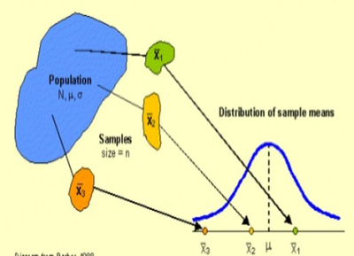
When we want information about the population proportion \(p\) of successes, we often take a simple random sample and use the sample proportion \(\hat p\) to estimate the unknown parameter \(p\). The sampling distribution of the sample proportion \(\hat p\) describes how the statistic varies in all possible samples of the same size from the population. In this lesson, students will explore the shape and variability of this distribution, and learn how to evaluate claims using the sampling distribution.
Standards
Computational Thinking in STEM 2.0
- Computational Data Practices
- [CT-DATA-1] Using computation to collect and create data
- [CT-DATA-6] Using computation to analyze data
- Computational Modeling and Simulation Practices
- [CT-MODEL-1] Using computational models to understand a complex phenomenon
- [CT-MODEL-2] Using computational models to hypothesize and test predictions
Activities
- 1. A quick review...
- 2. Assessing Normality
- 3. Investigating Normal Probability Plots using CODAP
- 4. When is the sampling distribution Normal(ish)?
- 5. Putting it all together!
Student Directions and Resources
Students will be able to:
- Calculate and interpret the mean and standard deviation of the sampling distribution of a sample proportion
- Determine if the sampling distribution of is approximately Normal
- Calculate and interpret the mean and standard deviation of the sampling distribution for a difference in sample proportions,
- Determine if the sampling distribution of a difference in proportions is approximately Normal
- Use a Normal distribution to calculate probabilities
1. A quick review...
Recall from Chapter 2, we had two main calculator functions that were used:
- normalcdf(lower bound, upper bound, mean, st dev): used to find the area under the Normal distribution between two bounds
- Example: IQ scores are normally distributed with mean 100 and a standard deviation of 15. Calculate the proportion of individuals that have IQ scores above 135.
- Solution: normalcdf(135, ∞, 100, 15) ≈ 0.0098 --> approx 1%
- invNorm(area under the Normal distribution to the LEFT of a z-score ("percentile"), mean, st dev): used to find the z-score or observation in a Normal distribution that is located at the nth percentile.
- Example: IQ scores are normally distributed with mean 100 and a standard deviation of 15. Mr Mills claims he scored in the 98th percentile on an IQ test. What is his IQ score?
- Solution: invNorm(0.98, 100, 15) ≈ 130.81
Answer the following questions below using your knowledge from Chapter 2
Question 1.1
Question 1.2
Calculate the following percentiles, given the z-score:
2. Assessing Normality
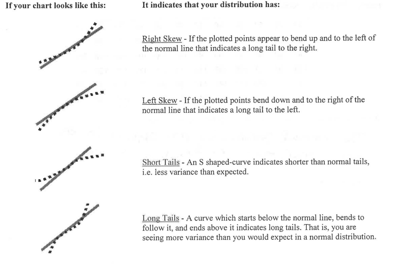
While normal distributions provide good models for some distributions of real data, the distributions of some the common variables are usually skewed and therefore distinctly non-normal. Examples include economic variables such as personal income and total sales of business firms, the survival times of cancer patients after treatment, and the lifetime of electronic devices. It is risky to assume that a distribution is normal without actually inspecting the data, so it is important to check a distribution for normality. You can assess the normality of a distribution by plotting the data using a dotplot, stemplot, or histogram or checking whether the data follow the 68–95–99.7 rule. However, just because a plot of the data looks normal, we can't say that the distribution is normal. For a better assessment of whether a data set follows a normal distribution, we can use a normal probability plot.
To assess the normality of a distribution from its normal probability plot, look at the plotted points, and see how well they fit the normal line. If they fit well, you can safely assume that your process data is normally distributed. If your plotted points don't fit the line well, but curve away from it in places, you may have a non normal distribution.
Question 2.1
If the points on your normal probability plot are fairly close to fitting a linear model, we can infer that the shape of the distribution is approximately ___________.
Skewed Right
Skewed Left
Normal
Uniform
Skewed Left
Normal
Uniform
Question 2.2
Why is it important to know whether or not the distribution of our data is approximately Normal?
3. Investigating Normal Probability Plots using CODAP
Follow the steps below to create a Normal Probability Plot! Answer the questions as you go through each step.
Question 3.1
Step 1: Sort the data in ascending order. To make sure you did this correctly, enter the smallest and largest value in this data set in the blanks below.
Question 3.2
Step 2: Calculate the percentile ("Percentile-Rank") for each data point. When you're done, give the percentile for data point #48 in the table.
Question 3.3
When you're done, take a screenshot of your normal probability plot and upload the screenshot below.
Upload files that are less than 5MB in size.
| File | Delete |
|---|---|
Upload files to the space allocated by your teacher.
Question 3.4
Describe what you see in the normal probability plot. Use these observations to make an inference about the shape of the distribution of this sample data.
4. When is the sampling distribution Normal(ish)?
Let's switch gears and look at sample proportions. The main question will investigate on this page:
When can we approximate the sampling distribution for proportions as Normal?
The model below allows you to select a sample size of your choice and set the population proportion to anything you want. We can use this model to evaluate claims about sample proportions in any context. You may want to drag the slider at the top to generate your samples more quickly. Scroll down to see instructions and questions.
Question 4.1
Set the model with parameters p = 0.15 and n = 5. Create an approximate sampling distribution. Describe the sampling distribution in context (Remember your SOCS!).
Question 4.2
Don't use the model yet. Make a prediction. What will happen to the sampling distribution if you make the true proportion higher (closer to p = 1)?
Question 4.3
OK, now use the model, change the proportion to something higher (like 0.8). How does the sampling distribution compare?
Question 4.4
Before using the model, make another prediction. What do you think will happen to the sampling distribution if we keep the proportion the same but increase the sample size from 5 to something higher (like 30)?
Question 4.5
Test your hypothesis by changing the sample size. How does the sampling distribution change?
Question 4.6
Which values for n and p will make the sampling distribution look the most similar to a Normal distribution? Perform some experiments using the model and report your findings here.
Question 4.7
Here's another model that can be used to explore the relationship between n and p. What are some advantages of using the NetLogo model compared to this simple model?
5. Putting it all together!
IMPORTANT - PLEASE READ
As you saw on the previous slide, the sampling distribution for \(\hat p\) depends on \(n\) and \(p\) . When \(p\) is closer to 0.5, and \(n\) is larger, the sampling distribution looks more Normal.
Here's a summary: Choose an SRS of size \(n\) from a population of size \(N\) with proportion \(p\) of successes. Let \(\hat p\) be the sample proportion of successes. Then, the following is true for the sampling distribution of \(\hat p\) (as long as the conditions are met):
| Formula/Attribute | Condition that must be met | |
| Shape: | approximately Normal | \(np \ge 10\) and \(n(1-p) \ge 10\) |
| Center: | \(\mu_\hat p = p\) | Random sampling (usually an SRS) |
| Spread: | \(\sigma_ \hat p = \sqrt \frac {p(1-p)}{n}\) | \(10n \leq N\) (10% condition) |
We will check these 3 conditions EVERY TIME we do a sampling problem about proportions.
Question 5.1
The Evanstonian is concerned about the effect of vaping and e-cigarettes at ETHS. The Evanstonian staff poll a simple random sample of 150 ETHS students and ask,
“Yes or No? Do you think that vaping (and/or e-cigarettes) are a problem at ETHS?”
Is the 10% condition satisfied? Why or why not? If so, calculate the standard deviation of the sampling distribution of \(\hat p\). Suppose it's known that 30% of students will say "yes" to this question.
Question 5.2
Suppose that 30% of all ETHS students respond “Yes” to this question. Let \(\hat p\) be the sample proportion of ETHS students who respond “Yes” to this question. What is the mean of the sampling distribution of \(\hat p\)?
Question 5.3
What is the shape of the sampling distribution of \(\hat p\)? Explain your reasoning and show work.
Question 5.4
What is the probability that, in a random sample of 150 ETHS students, less than 25% will respond "Yes". (Note: You've shown that this data can be approximated as normal, and you have calculated the mean and standard deviation of that distribution. This is now the sort of problem that you did waaaay back in chapter 2!)
Upload files that are less than 5MB in size.
| File | Delete |
|---|---|
Upload files to the space allocated by your teacher.