What is the parameter of interest? What symbol is used to represent this value?
Unit Overview
In this unit, students will explore the beginning of statistical inference - making conclusions about a population based on data from a sample. Sampling distributions are the foundation of inference when data are produced by random sampling.
Standards
Computational Thinking in STEM 2.0
- Computational Data Practices
- [CT-DATA-1] Using computation to collect and create data
- [CT-DATA-6] Using computation to analyze data
- Computational Modeling and Simulation Practices
- [CT-MODEL-1] Using computational models to understand a complex phenomenon
- [CT-MODEL-2] Using computational models to hypothesize and test predictions
Underlying Lessons
- Lesson 1. Introduction - What is a Sampling Distribution?
- Lesson 2. Bias and Variability
- Lesson 3. Assessing Normality
- Lesson 4. Applications using Sample Proportions
- Lesson 5. The Central Limit Theorem
Lesson 1 Overview
The purpose of this lesson is to give students hands-on experience with creating and using sampling distributions. Once the concept is understood, the lesson asks them to use sampling distributions to evaluate a claim (based on informal reasoning, we don’t introduce p-value yet). The sampling distributions will be generated using a NetLogo model. After using the model as it was created, students are asked to modify the NetLogo model to generate a modified sampling distribution.
Lesson 1 Activities
- 1.1. Statistic vs. Parameter
- 1.2. Sampling by hand
- 1.3. What is a Sampling Distribution?
- 1.4. Sampling Distributions on a larger scale
- 1.5. Using a Sampling Distribution to reason about data
- 1.6. Final Thoughts
1.0. Student Directions and Resources
SWBAT (students will be able to): Define/recognize/use/describe the following:
- Parameter vs. Statistic
- Sampling Distribution
- Distribution of a Sample
- Distribution of a Population
SWBAT Evaluate claims using sampling distributions
1.1. Statistic vs. Parameter
A statistic is a number that describes some characteristic of a sample.
A parameter is a number that describes some characteristic of a population.
The table below shows three commonly used statistics and their corresponding parameters. These symbols are widely used in statistics and you are expected to know and use these symbols and terms. The symbol for sample mean is read "x bar" and the symbol for sample proportion is read "p hat." PLEASE get out your notebook and write down the following symbols and their meanings:
| Sample Statistic | Population Parameter | |
| \(\bar x\) (sample mean) | estimates | \(\mu\) (population mean) |
| \(\hat p\) (sample proportion) | estimates | \(p\) (population proportion) |
| sx (sample st. dev) | estimates | \(\sigma\) (population st. dev) |
Use the following scenario for the questions below:
From a large group of people who signed a card saying they intended to quit vaping, 1000 people were selected at random. It turned out that 210 (21%) of these individuals had not vaped over the past 6 months.
Question 1.1.1
Question 1.1.2
What is the statistic obtained from the sample? What symbol is used to represent this value?
1.2. Sampling by hand
Since we do a lot of small group work in AP Statistics, we’ve decided to sample 2 students from a group of 4 and take the average of their scores to get an estimate for how well students in this group performed on the exam. **Note: usually people wouldn’t use a sample and population this small, but we’re starting small to help you visualize what we’re doing.**
For this scenario, our population will be 4 students with the following scores: Alexis - 3, Bert - 4, Chris - 5, Devin - 5
Question 1.2.1
How many samples of size 2 can be taken from this population?
Question 1.2.2
What is the parameter of interest for this situation?
Question 1.2.3
What statistic are we using to estimate the parameter of interest for this situation?
Question 1.2.4
Do you think taking a sample this size from this population effectively estimates the mean score of the population?
1.3. What is a Sampling Distribution?
Since we do a lot of small group work in AP Statistics, we’ve decided to sample 2 students from a group of 4 and take the average of their scores to get an estimate for how well students in this group performed on the exam.
For this scenario, our population will be 4 students with the following scores: 3,4,5,5
Use the NetLogo model below to simulate choosing two students (n=2) at a time from this population (N=4).
1) Click "setup" to start the model. If you are bothered by a person being cutoff on the edge of the screen, click "setup" again.
2) Click "collect sample" to choose your first sample, and record your results in the table below before pressing the button again.
3) Continue pressing "collect sample" and entering data into the table below until all possible samples have been chosen.
*Note: you may have to add additional rows to the data table.
Question 1.3.1
Calculate the sample mean for all possible samples of size 2 from this population.
Question 1.3.2
Create a dotplot of your results from question #2. Create your sketch below.
Note: Draw your sketch in the sketchpad below
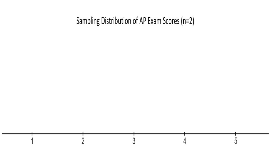
Question 1.3.3
In most real-life situations, we cannot create the dotplot of all possible samples of size n from the entire population (size N). Why not?
1.4. Sampling Distributions on a larger scale
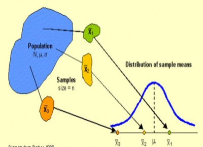
What you created on the previous page was the sampling distribution of AP scores for that group of 4 students. You took all six possible samples (n=2) from a population of four students (N=4). Sampling distributions are an important concept in Statistics and understanding what they are is the key to everything we do for the rest of the year.
A sampling distribution shows all possible samples of size n taken from a population of size N. In real-life scenarios, we don't create the entire sampling distribution by hand, or even using a computer, because our population is much larger (or it's size is unknown). For illustrative purposes we will use a NetLogo model to simulate taking samples of AP Statistics exam scores from last year. There were 48 students in our classes last year, and we’ll take samples of 2 students at a time.
Here's the new scenario:
Question 1.4.1
Click "setup" and then "collect sample". What did the model do?
Question 1.4.2
Press the "collect sample" button 30 times. Drag the word "Mean" from the table to the horizontal axis of the empty graph. The graph is starting to take shape, but it cannot be called a sampling distribution yet... Why not?
Question 1.4.3
A school administrator took a sample of 2 AP statistics students and found their average AP test score to be 1.5. Based on that sample, the Administrator is claiming that the mean test score for all AP stats students at ETHS is 1.5. Do you have substantial evidence to refute their claim? You just created a statistical model - use it to explain to the administrator that their estimate is probably wrong.
Question 1.4.4
What was wrong with the administrator's sample?
1.5. Using a Sampling Distribution to reason about data
We ran the model from the previous page until we collected every possible sample of 2 students. Below you can see the ENTIRE sampling distribution for our situation (n = 2, N = 48 students).
Question 1.5.1
On the left side of the screen you see a table. Click on one of the cells in the row with "index" 17. This should highlight one single dot on the dotplot. Explain what that dot represents in the context of the situation.
Question 1.5.2
Suppose an administrator is claiming that the true Mean score of the population is 3.2. Do you have convincing evidence to refute their claim? Explain.
1.6. Final Thoughts
Question 1.6.1
What is at least one big idea that you learned about sampling distributions in this lesson? Explain.
Question 1.6.2
Pick any computational tool/activity that you have used in this lesson. Briefly describe the tool and explain how you used it to learn.
Question 1.6.3
Indicate how much you agree or disagree with the following statement:
I enjoyed learning with the computational tools/activities in this lesson.
Strongly disagree
Disagree
In the middle / I don't know
Agree
Strongly agree
Disagree
In the middle / I don't know
Agree
Strongly agree
Question 1.6.4
Indicate how much you agree or disagree with the following statement:
I found this lesson more engaging compared to my other lessons without computational tools/activities,
Strongly disagree
Disagree
In the middle / I don't know
Agree
Strongly agree
Disagree
In the middle / I don't know
Agree
Strongly agree
Question 1.6.5
Indicate how much you agree or disagree with the following statement:
Compared to lessons without computational tools/activities, I found this lesson more challenging.
Strongly disagree
Disagree
In the middle / I don't know
Agree
Strongly agree
Disagree
In the middle / I don't know
Agree
Strongly agree
Question 1.6.6
Indicate how much you agree or disagree with the following statement:
I feel that I successfully learned the content of this lesson.
Strongly disagree
Disagree
In the middle / I don't know
Agree
Strongly agree
Disagree
In the middle / I don't know
Agree
Strongly agree
Question 1.6.7
Indicate how much you agree or disagree with the following statement:
I felt stressed by the computational tools/activities we have done in this lesson.
Strongly disagree
Disagree
In the middle / I don't know
Agree
Strongly agree
Disagree
In the middle / I don't know
Agree
Strongly agree
Question 1.6.8
Is anything that you learned in this lesson relevant to your personal aspirations? If yes, please explain.
Lesson 2 Overview
Students modify their sampling distribution model to see how the sampling distributions of biased and non-biased estimators compare and to investigate the effects of sample size on variability in a sampling distribution. Extra emphasis is given to the difference between bias and variability.
Lesson 2 Activities
- 2.1. Intro to a new sampling model
- 2.2. Biased Vs. Non-Biased Estimators
- 2.3. Bias
- 2.4. Sample size and variability
- 2.5. Bias vs. Variability
- 2.6. Reflection
2.0. Student Directions and Resources
SWBAT:
Understand/use/define Bias vs. Variability
Understand/use/define the relationship between sample size and variability
2.1. Intro to a new sampling model
In the previous lesson we learned about Sampling Distributions. We specifically looked at a sampling distribution of MEANS. In this lesson we're going to use the same model that we used in the previous lesson to create and compare sampling distributions for a few different statistics. (note all sampling distributions created in this lesson are actually approximations, they are not complete, but they are perfectly good for our purposes)
Scroll down to see instructions and questions for this page.
Question 2.1.1
First, we'll create the same sampling distribution that we created yesterday. Use the model above to create the sampling distribution for the mean scores of samples of 2 students (n=2) taken from a population of 48 students (N=48).
1) Set the slider and click "setup" and "collect samples." The sampling will happen faster if you pull the "model speed" slider all the way to the right.
2) Click the button that says "tables" in the upper left, then "data set" in order to see your data table. You can drag it around in the CODAP window to wherever you want it.
3) Now we'll set up the graph. First, click the "graph" button in the top left. Then click the "click here" along the x-axis and select "mean."
4) We're also going to find the mean of the data in this graph (That is, the mean of all the means from each sample). To do that click on the ruler to the right of the graph and check "mean." There should now be a line in the middle of your sampling distribution for the mean, and you can hover over it to find out its value.
The mean score for our population of 48 students is 3.4. Is your mean close to that value?
2.2. Biased Vs. Non-Biased Estimators
Now we're going to do the same thing, except instead of calculating the mean score for our sample, we're going to calculate the MAXIMUM score of our sample. We (Mr. Mickelson and Mr. Mills) made this model, so we can change it in order to explore a different statistic. We're going to change the model to find the maximum of each sample.
Note: If you need to start fresh just reload the page and everything will reset.
a) Underneath the model window is a tab called "netLogo Code". Click on that to open the code. Don't freak out, we're just going to make one little change!
b) Scroll down to find line 29. You can see the line numbers on the left side of the workspace.
c) In lines 30 and 31 you should see the word "Mean." In both places, change the word Mean to the word Max.
d) Press recompile code at the top of the workspace.
e) Click setup and collect samples. This time the model will take the maximum value from each sample.
e) Click "tables," the "data set" again. Click "graph" and this time put the "Max" on the axis of the graph.
f) Add the mean to your graph of sample maximums (click the ruler, then check "Mean").
Question 2.2.1
For our population, what is the actual maximum? Is the mean of this sampling distribution close to that value?
Question 2.2.2
Now erase that data (either with the trashcan icon under "tables" or refreshing the page) and do the same thing using the minimum statistic (just repeat what you did for Max, just use the word Min).
Is the mean of this sampling distribution the same as the actual value of the population minimum?
2.3. Bias
On the previous pages you probably noticed that the center of the "Mean" sampling distribution lined up pretty closely with the center of the actual population distribution. However, the center of the "Max" and "Min" sampling distribution did not match up with the actual maximum and minimum of the population. The statistics "Max" and "Min" are examples of BIASED estimators. The mean of their sampling distribution is not equal to the actual value of the population parameter.
Question 2.3.1
Do you think the mean is a biased estimator? Explain your reasoning.
Question 2.3.2
On the next page we'll use the same model but increase the size of our sample (n). What do you think will happen to the sampling distribution? How will that show up in the model?
Question 2.3.3
On the next page you'll be asked to use the model to see how sample size affects the variability of the sampling distribution.
Make a plan for how you'll use the model to investigate this question.
2.4. Sample size and variability
Here's the same model, but now we're back to calculating means. Scroll down for instructions!
Question 2.4.1
Use your plan and investigate how changing the sample size affects the variability of the sampling distribution (you can show the standard deviation on your graphs in the same way that we showed the mean, go back to page 1 if you need to!). Was your prediction on the previous page correct?
Question 2.4.2
By what factor do you need to increase the sample size in order for the standard deviation to be cut in half?
Question 2.4.3
By what factor do you think you need to increase sample size in order to reduce the standard deviation to 1/3 of it's value?
Question 2.4.4
Based on you answers to the previous questions, make a guess about the formula for the standard deviation of a sampling distribution. In other words, what effect does sample size have on standard deviation and how does this show up in the formula? Use your knowledge from previous math courses to answer this question!
Question 2.4.5
When we're taking samples in real life in order to estimate the true value of a parameter, is it better to have more or less variation?
2.5. Bias vs. Variability
This is just a page to put together your understanding of bias and variability. A lot of times students say "more biased" when they really mean "less variable", so this is a pretty important thing to nail down!
Question 2.5.1
On pages 2-3 you learned about bias. On page 4 you learned about variability. Explain the difference between bias and variability in a way that a freshman could understand. You are welcome to use your book and the internet for more definitions and illustrations (I think your book has a really useful graphic on page 481).
Question 2.5.2
Ideally, we want the variation in our sampling distribution to be as _______ as possible.
High
Medium
Low
Medium
Low
Question 2.5.3
Two graduate students are studying the effects of a new cancer drug. Student A took a sample of size 10 from the population, while student B took a sample of size 30. Whose results will be more precise? Why? What do we mean by 'precise'?
2.6. Reflection
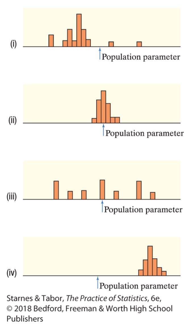
(Use the figure below for questions 1 and 2)
The figure shows approximate sampling distributions of 4 different statistics intended to estimate the same parameter.
Question 2.6.1
Which statistics are unbiased estimators? Justify your answer.
Question 2.6.2
Which statistic does the best job of estimating the parameter? Explain your answer.
Question 2.6.3
The Evanstonian is collecting responses for an opinion poll. The editor suggests that they increase their sample size. The statistical reason for increasing the sample size of the opinion poll is to reduce _____________________________.
bias of the estimates made from the data collected in the poll.
variability of the estimates made from the data collected in the poll.
effect of nonresponse on the poll.
variability of opinions in the sample.
variability of opinions in the population.
variability of the estimates made from the data collected in the poll.
effect of nonresponse on the poll.
variability of opinions in the sample.
variability of opinions in the population.
Lesson 3 Overview
When we want information about the population proportion \(p\) of successes, we often take a simple random sample and use the sample proportion \(\hat p\) to estimate the unknown parameter \(p\). The sampling distribution of the sample proportion \(\hat p\) describes how the statistic varies in all possible samples of the same size from the population. In this lesson, students will explore the shape and variability of this distribution, and learn how to evaluate claims using the sampling distribution.
Lesson 3 Activities
- 3.1. A quick review...
- 3.2. Assessing Normality
- 3.3. Investigating Normal Probability Plots using CODAP
- 3.4. When is the sampling distribution Normal(ish)?
- 3.5. Putting it all together!
3.0. Student Directions and Resources
Students will be able to:
- Calculate and interpret the mean and standard deviation of the sampling distribution of a sample proportion
- Determine if the sampling distribution of is approximately Normal
- Calculate and interpret the mean and standard deviation of the sampling distribution for a difference in sample proportions,
- Determine if the sampling distribution of a difference in proportions is approximately Normal
- Use a Normal distribution to calculate probabilities
3.1. A quick review...
Recall from Chapter 2, we had two main calculator functions that were used:
- normalcdf(lower bound, upper bound, mean, st dev): used to find the area under the Normal distribution between two bounds
- Example: IQ scores are normally distributed with mean 100 and a standard deviation of 15. Calculate the proportion of individuals that have IQ scores above 135.
- Solution: normalcdf(135, ∞, 100, 15) ≈ 0.0098 --> approx 1%
- invNorm(area under the Normal distribution to the LEFT of a z-score ("percentile"), mean, st dev): used to find the z-score or observation in a Normal distribution that is located at the nth percentile.
- Example: IQ scores are normally distributed with mean 100 and a standard deviation of 15. Mr Mills claims he scored in the 98th percentile on an IQ test. What is his IQ score?
- Solution: invNorm(0.98, 100, 15) ≈ 130.81
Answer the following questions below using your knowledge from Chapter 2
Question 3.1.1
Calculate the z-scores for each of the following percentiles:
Question 3.1.2
Calculate the following percentiles, given the z-score:
3.2. Assessing Normality
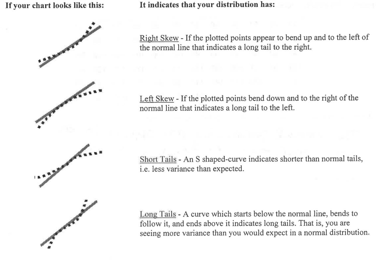
While normal distributions provide good models for some distributions of real data, the distributions of some the common variables are usually skewed and therefore distinctly non-normal. Examples include economic variables such as personal income and total sales of business firms, the survival times of cancer patients after treatment, and the lifetime of electronic devices. It is risky to assume that a distribution is normal without actually inspecting the data, so it is important to check a distribution for normality. You can assess the normality of a distribution by plotting the data using a dotplot, stemplot, or histogram or checking whether the data follow the 68–95–99.7 rule. However, just because a plot of the data looks normal, we can't say that the distribution is normal. For a better assessment of whether a data set follows a normal distribution, we can use a normal probability plot.
To assess the normality of a distribution from its normal probability plot, look at the plotted points, and see how well they fit the normal line. If they fit well, you can safely assume that your process data is normally distributed. If your plotted points don't fit the line well, but curve away from it in places, you may have a non normal distribution.
Question 3.2.1
If the points on your normal probability plot are fairly close to fitting a linear model, we can infer that the shape of the distribution is approximately ___________.
Skewed Right
Skewed Left
Normal
Uniform
Skewed Left
Normal
Uniform
Question 3.2.2
Why is it important to know whether or not the distribution of our data is approximately Normal?
3.3. Investigating Normal Probability Plots using CODAP
Follow the steps below to create a Normal Probability Plot! Answer the questions as you go through each step.
Question 3.3.1
Step 1: Sort the data in ascending order. To make sure you did this correctly, enter the smallest and largest value in this data set in the blanks below.
Question 3.3.2
Step 2: Calculate the percentile ("Percentile-Rank") for each data point. When you're done, give the percentile for data point #48 in the table.
Question 3.3.3
When you're done, take a screenshot of your normal probability plot and upload the screenshot below.
Upload files that are less than 5MB in size.
| File | Delete |
|---|---|
Upload files to the space allocated by your teacher.
Question 3.3.4
Describe what you see in the normal probability plot. Use these observations to make an inference about the shape of the distribution of this sample data.
3.4. When is the sampling distribution Normal(ish)?
Let's switch gears and look at sample proportions. The main question will investigate on this page:
When can we approximate the sampling distribution for proportions as Normal?
The model below allows you to select a sample size of your choice and set the population proportion to anything you want. We can use this model to evaluate claims about sample proportions in any context. You may want to drag the slider at the top to generate your samples more quickly. Scroll down to see instructions and questions.
Question 3.4.1
Set the model with parameters p = 0.15 and n = 5. Create an approximate sampling distribution. Describe the sampling distribution in context (Remember your SOCS!).
Question 3.4.2
Don't use the model yet. Make a prediction. What will happen to the sampling distribution if you make the true proportion higher (closer to p = 1)?
Question 3.4.3
OK, now use the model, change the proportion to something higher (like 0.8). How does the sampling distribution compare?
Question 3.4.4
Before using the model, make another prediction. What do you think will happen to the sampling distribution if we keep the proportion the same but increase the sample size from 5 to something higher (like 30)?
Question 3.4.5
Test your hypothesis by changing the sample size. How does the sampling distribution change?
Question 3.4.6
Which values for n and p will make the sampling distribution look the most similar to a Normal distribution? Perform some experiments using the model and report your findings here.
Question 3.4.7
Here's another model that can be used to explore the relationship between n and p. What are some advantages of using the NetLogo model compared to this simple model?
3.5. Putting it all together!
IMPORTANT - PLEASE READ
As you saw on the previous slide, the sampling distribution for \(\hat p\) depends on \(n\) and \(p\) . When \(p\) is closer to 0.5, and \(n\) is larger, the sampling distribution looks more Normal.
Here's a summary: Choose an SRS of size \(n\) from a population of size \(N\) with proportion \(p\) of successes. Let \(\hat p\) be the sample proportion of successes. Then, the following is true for the sampling distribution of \(\hat p\) (as long as the conditions are met):
| Formula/Attribute | Condition that must be met | |
| Shape: | approximately Normal | \(np \ge 10\) and \(n(1-p) \ge 10\) |
| Center: | \(\mu_\hat p = p\) | Random sampling (usually an SRS) |
| Spread: | \(\sigma_ \hat p = \sqrt \frac {p(1-p)}{n}\) | \(10n \leq N\) (10% condition) |
We will check these 3 conditions EVERY TIME we do a sampling problem about proportions.
Question 3.5.1
The Evanstonian is concerned about the effect of vaping and e-cigarettes at ETHS. The Evanstonian staff poll a simple random sample of 150 ETHS students and ask,
“Yes or No? Do you think that vaping (and/or e-cigarettes) are a problem at ETHS?”
Is the 10% condition satisfied? Why or why not? If so, calculate the standard deviation of the sampling distribution of \(\hat p\). Suppose it's known that 30% of students will say "yes" to this question.
Question 3.5.2
Suppose that 30% of all ETHS students respond “Yes” to this question. Let \(\hat p\) be the sample proportion of ETHS students who respond “Yes” to this question. What is the mean of the sampling distribution of \(\hat p\)?
Question 3.5.3
What is the shape of the sampling distribution of \(\hat p\)? Explain your reasoning and show work.
Question 3.5.4
What is the probability that, in a random sample of 150 ETHS students, less than 25% will respond "Yes". (Note: You've shown that this data can be approximated as normal, and you have calculated the mean and standard deviation of that distribution. This is now the sort of problem that you did waaaay back in chapter 2!)
Upload files that are less than 5MB in size.
| File | Delete |
|---|---|
Upload files to the space allocated by your teacher.
Lesson 4 Overview
When we want information about the population proportion of successes, we often take a simple random sample and use the sample proportion to estimate the unknown parameter . The sampling distribution of the sample proportion describes how the statistic varies in all possible samples of the same size from the population. In this lesson, students will explore the shape and variability of this distribution, and learn how to evaluate claims using the sampling distribution.
Lesson 4 Activities
- 4.1. Thinking about our Context
- 4.2. Introducing our Context
- 4.3. Apply - evaluate claims using the sampling distribution
- 4.4. Introduction to sampling from 2 populations
- 4.5. Setting up for 2 samples
- 4.6. Carrying out the 2 Samples and calculating the difference in sample proportions
- 4.7. Formulas and Calculations
- 4.8. Reminder about the need to collect and analyze statistics
- 4.9. Practice with 2 proportions
4.0. Student Directions and Resources
Students will be able to:
- Calculate and interpret the mean and standard deviation of the sampling distribution of a sample proportion \(\hat p\)
- Determine if the sampling distribution of \(\hat p\) is approximately Normal
- Calculate and interpret the mean and standard deviation of the sampling distribution for a difference in sample proportions, \(\hat p_1 - \hat p_2\)
- Determine if the sampling distribution of a difference in proportions, \(\hat p_1 - \hat p_2\) , is approximately Normal
- Use a Normal distribution to calculate probabilities involving \(\hat p\) and \(\hat p_1 - \hat p_2\)
4.1. Thinking about our Context
One thing that police do is make traffic stops. There are many different reasons that the police might choose to pull someone over and in some cases give the driver a ticket. Is their decision affected by gender? race? socio-economic status? time of day? type of car? Statistics is one way to answer these questions but it can also be used to purposely mislead people about the answers to these questions.
"There are three types of lies - lies, damn lies, and statistics" (attributed to Mark Twain, maybe aprocryphal)
We’re going to look at some Evanston Police Department (EPD) data about traffic stops between 1/1/2020 and 7/23/2020 and try to come up with some truthful answers.
Question 4.1.1
How many total traffic stops do you think that EPD made in the 6.75 months between 1/1/20 and 7/23/20? I realize you have no great way of knowing, take a guess!
4.2. Introducing our Context
Here is the data, there were 22687 total traffic stops as reported by EPD. There are lots of different questions that we might want to answer based off of this data. As you know, over the past many years Police Departments have been under scrutiny for how they treat people of color, specifically black people. In the Summer of 2020, the murder of George Floyd at the hands of the police was the latest in a string of innocent black lives lost in their interactions with police (https://www.bbc.com/news/world-us-canada-52905408). The ensuing protests and the Black Lives Matter Movement have put police treatment of black Americans in the spotlight. For that reason, we will specifically focus on data about traffic stops of black drivers throughout this lesson. Let's take a look at Data from Evanston. Clearly this could be an issue for any race, or gender, or a lot of other things, but for the purpose of this lesson we'll focus specifically on black vs. non-black drivers in Evanston.
Remember, this is traffic stops by EPD from 1/1/20 - 7/23/20 broken down by race.
| Race | Number |
| White | 12407 |
| Black | 6887 |
| Hispanic | 1784 |
| Asian | 1465 |
| Unknown | 144 |
| Total | 22687 |
See below for questions and instructions.
Question 4.2.1
Someone looks at this data and concludes that EPD is biased against white people. Do you agree? How would you use this data to support or refute their claim?
Question 4.2.2
What other information do you think is needed in order to investigate the idea that EPD is disproportionately stopping one race of driver?
Question 4.2.3
Calculate the proportion of traffic stops in which the driver was black.
Question 4.2.4
Set the population proportion slider to match your answer in the previous question. When you click "setup" button and then the “take sample” button the model will take an SRS of 5 traffic stops and report the proportion of drivers who identify as black. Take a few samples. Do you get proportions close to the actual value? Explain why you do or do not.
Question 4.2.5
On the next page you're going to do some work with sampling distributions. Define the term "sampling distribution" in one sentence.
Question 4.2.6
Before we get too deep into this, let's acknowledge that this is a very complicated issue. The how and why of traffic stops is complicated. Understanding that there are no right answers, what are some possible problems that exist with this data before we do anything to it?
4.3. Apply - evaluate claims using the sampling distribution
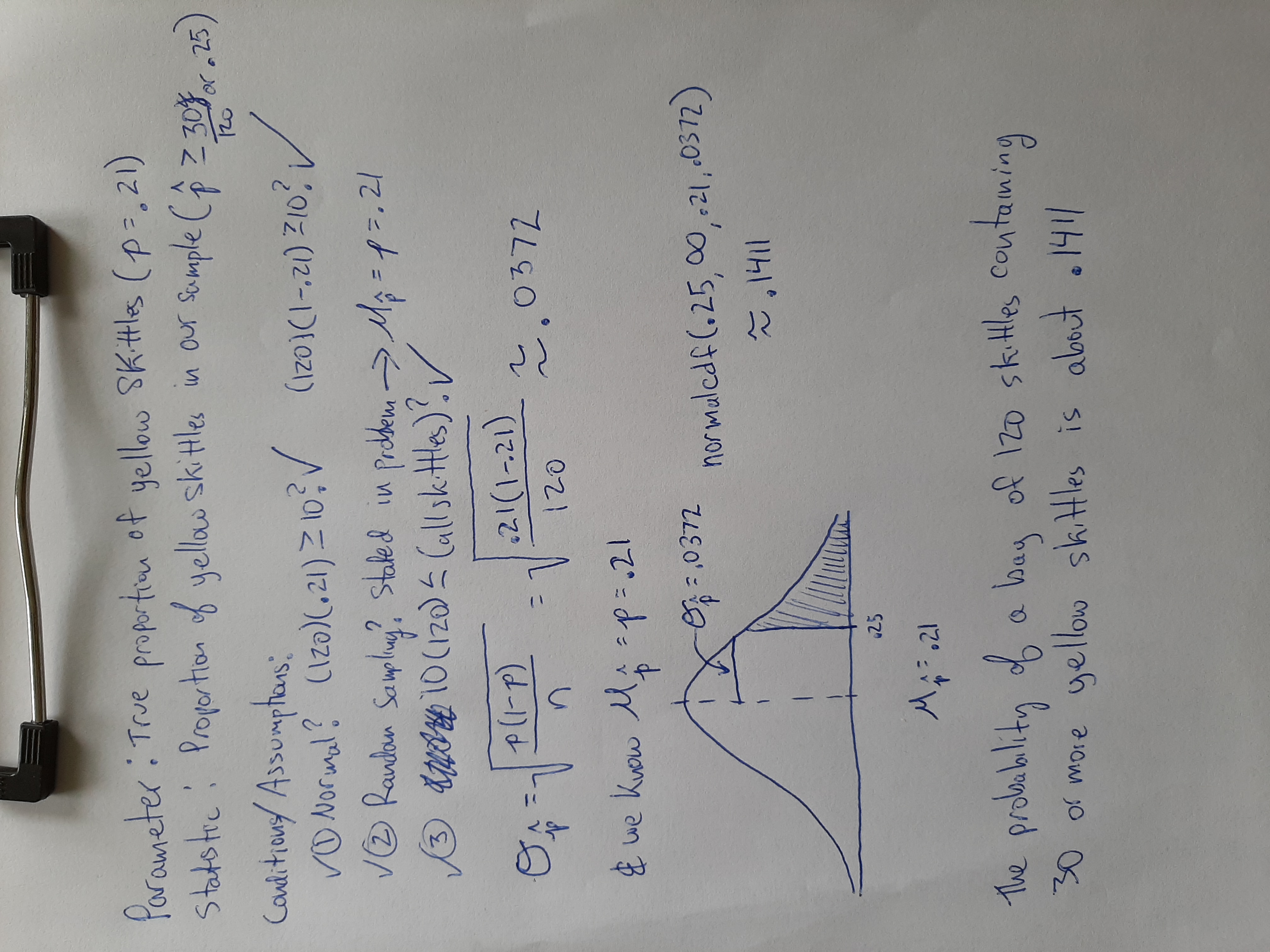
Below are a few additional questions related to sampling distributions for proportions. These are the sorts of questions that you'll be expected to answer on an AP test. Be sure to check all necessary conditions and show all work. Do your work on paper and upload a scanned image for the questions below. See the example below for what an exemplary response looks like for these types of problems.
Example problem and solution: Suppose it is known that 21% of all Skittles produced are yellow. We will also assume that every bag of Skittles is a simple random sample from that entire population. Suppose you purchase a bag containing 120 Skittles. What is the probability of that bag containing 30 or more yellow Skittles?
Question 4.3.1
In a congressional district, 55% of registered voters are Democrats. Suppose we take a random sample of 100 voters from this congressional district. What is the probability of getting less than 50% Democrats in a random sample of size 100?
Upload files that are less than 5MB in size.
| File | Delete |
|---|---|
Upload files to the space allocated by your teacher.
Question 4.3.2
In July 2020, the Chicago Tribune asked a random sample of 750 Chicago residents. "Do you wear a face covering in public?" Based on a previous study by the IDPH, we know that 50% of ALL Chicago residents actually wear a face covering in public. Let \(\hat p\) be the sample proportion who say that they wear a face covering in public. What is the probability that, in a random sample of 750, more than 75% will respond "Yes (I wear a face covering in public)"?
Upload files that are less than 5MB in size.
| File | Delete |
|---|---|
Upload files to the space allocated by your teacher.
4.4. Introduction to sampling from 2 populations
We're coming back to our EPD data. A newspaper article claims that the proportion of traffic stops for black residents in Evanston (p1) is HIGHER than the proportion of black residents in Evanston (p2).
Question 4.4.1
If the claim is true what could that suggest about racial bias in EPD?
Question 4.4.2
The idea that Police aren't always fair in carrying out their duties can bring up a lot of feelings and experiences. Do you have any personal thoughts or experiences about this topic that you'd like to share?
Question 4.4.3
What would it mean if p1 = p2?
4.5. Setting up for 2 samples
We’re lucky that the Evanston Police Department keeps these sorts of records AND makes them available to the public. We don't have to use sampling in order to estimate the proportion of traffic stops that involve black drivers. But this is a lesson about sampling, SO WE'RE GOING TO PRETEND!
Let’s say we didn’t have all the data that we do have, so we HAD to use random sampling in order to investigate. For the remainder of this lesson, we’re going to pretend that we don’t have the full data, and we’re going to generate random samples in order to simulate real-world sampling.
We’re going to have to use sampling to estimate two different proportions:
1. The proportion of all traffic stops that are of black drivers
2. The proportion of Evanston residents who are black
There are a total of 72,836 residents in Evanston and 22,687 traffic stops made.
Question 4.5.1
Using our omnipotence, we believe that the proportion of black drivers stopped in traffic stops is about 30%. What is the largest sample size you could use to estimate the true proportion of black drivers stopped in traffic stops? Show your calculations. What is the smallest sample size you could use? Jot down these numbers as you're going to need it later on!
Question 4.5.2
Once again, we'll use our omnipotence to guess that the true proportion of black residents in Evanston is about 17%. What is the largest sample you could take from the entire population in Evanston and still meet all of our conditions? What is the smallest sample size you could use? Show calculations. Jot down this number as you're going to need it later on!
Question 4.5.3
There's something obviously unrealistic in our pretend scenario. In real life we might not have any idea about the true proportions. What do you think you would do in that case? (we'll answer this question in the next chapter!)
4.6. Carrying out the 2 Samples and calculating the difference in sample proportions
What we really care about here is the DIFFERENCE between our two proportions.
Let p1 be the true proportion of Evanston black drivers stopped in traffic stops.
Let p2 be the true proportion of all black residents in Evanston.
Question 4.6.1
What does it mean in context if p1 - p2 is POSITIVE?
Question 4.6.2
What does it mean in context if p1 - p2 is ZERO?
Question 4.6.3
What does it mean in context if p1 - p2 is NEGATIVE?
4.7. Formulas and Calculations
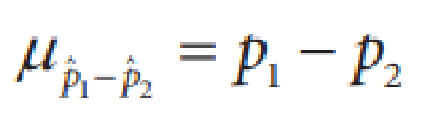
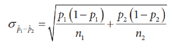
Here are the formulas for the standard deviation and the mean of a difference between two proportions. Use the model, the known population proportions, and the sampling sizes you calculated before to carry out sampling for both proportions. Scroll down for detailed instructions.
Question 4.7.1
Calculate the mean (\(\mu_{\hat {p_1} - \hat {p_2}}\)) and standard deviation (\(\sigma_{\hat {p_1} - \hat {p_2}}\)). This is the center and spread of our sampling distribution for the difference in proportions.
Question 4.7.2
Set the population proportion to our actual value for proportion of traffic stops of black drivers (0.30). Set the sample size slider to the number you calculated on page 7 for the smallest allowable sample size. Collect a sample, and record your sample proportion (\(\hat p_1\)) here.
Question 4.7.3
Set the population proportion to our actual value for proportion of black resisdents in Evanston (0.17). Set the sample size slider to the number you calculated on page 7 for the smallest allowable sample size. Collect a sample, and record your sample proportion (\(\hat p_2\)) here.
Question 4.7.4
What conclusion(s) would you draw BASED ON YOUR DATA? (We would like you to draw a conclusion about the population from your sample results, using the Normal distribution)
4.8. Reminder about the need to collect and analyze statistics
Here's the real values for p1 and p2.
p1=0.3057
p2=0.17
Question 4.8.1
Calculate the value of \(p_1 - p_2\)
Question 4.8.2
Explain what this difference in proportions means in real life, in a way that any high school student could understand.
Question 4.8.3
How close was your estimate based on random sampling?
Question 4.8.4
We've been pretending that we didn't have all of the data, so we had to use random sampling in order to estimate our population proportions. Explain why in real life we would NEED to use random sampling to do a similar analysis in a different situation.
Question 4.8.5
Based on this data it seems that black drivers are disproportionately pulled over in Evanston. How do you feel about that?
Question 4.8.6
What additional data could we use to explore this issue more deeply?
and/Or
What are some things that we could do to begin to address this?
and/Or
What are some other questions that we could investigate using this (or other) data?
4.9. Practice with 2 proportions
Suppose we want to investigate the effectiveness of two potential COVID-19 vaccines. We will call these "Vaccine 1" and "Vaccine 2".
During Phase 3 trials of the vaccine development process, thousands of volunteers are randomly assigned one of the two vaccines. After 30 days, researchers take blood samples to detect if antibodies are present. The presence of antibodies would indicate that the vaccine has been effective at preventing the individual from experiencing moderate to severe COVID-19 symptoms. The table below shows the results of some randomly selected volunteers from each vaccine trial.
| Antibodies present | No antibodies present | |
| Vaccine 1 | 53 | 22 |
| Vaccine 2 | 59 | 16 |
Question 4.9.1
Identify each of the following, using the table above : \(n_1, n_2, \hat p_1, \hat p_2\)
Question 4.9.2
Based on the sample results, which vaccine seems to be more effective? Provide evidence to support your reasoning.
Question 4.9.3
Let's analyze the difference between these two sample proportions. Calculate \(\hat p_1 - \hat p_2\)
Question 4.9.4
For the standard deviation formula, we need to think back to our work with combining random variables in Chapter 6. Remember: you have a formula for the standard deviation of \(\hat p_1 - \hat p_2\) on your formula sheet!
Calculate this value for our scenario using your answers from question 8.1
Question 4.9.5
Later on, we found out that the two vaccines are equally effective. What is the probability of observing a difference in sample proportions greater than the one shown in the table? Be sure to check the Normal condition for each population.
Lesson 5 Overview
Students will explore the relationship between the shape of the population distribution, the sample size and the shape of the sampling distribution.
Central Limit Theorem demonstrates relations between population distributions and their sample mean distributions as well as the effect of sample size on this relation. In this model, a population is distributed by some variable, for instance by their total assets in thousands of dollars. The population is distributed randomly -- not necessarily 'normally' -- but sample means from this population nevertheless accumulate in a distribution that approaches a normal curve. The program allows for repeated sampling of individual specimens in the population
Lesson 5 Activities
- 5.1. Exploring Central Limit Theorem in a NetLogo model
- 5.2. Exploring different population distributions
- 5.3. Reflection
- 5.4. Applications
- 5.5. Central Limit Theorem applications
- 5.6. Difference between Two Sample Means
- 5.7. Another difference of sample means problem
- 5.8. Some Final Thoughts
5.0. Student Directions and Resources
By the end of this lesson, you should be able to:
- Explain how the shape of the sampling distribution of is affected by the shape of the population distribution and the sample size (aka, The Central Limit Theorem)
- Explain why the Central Limit Theorem is one of the fundamental theorems in statistics
- Calculate the mean and standard deviation of the sampling distribution of a sample mean \(\bar x\) and interpret the standard deviation
- Calculate the mean and standard deviation of the sampling distribution of a difference in sample means \(\bar x_1- \bar x_2\) and interpret the standard deviation
- Determine if the sampling distribution of \(\bar x_1- \bar x_2\) is approximately Normal
- If appropriate, use a Normal distribution to calculate probabilities involving \(\bar x\) and \(\bar x_1- \bar x_2\)
5.1. Exploring Central Limit Theorem in a NetLogo model
Use the NetLogo model below to answer the questions.
Question 5.1.1
In the NetLogo model above, press "SETUP" and then "Preset 1". Describe the shape of this distribution.
Question 5.1.2
Set the sample-size slider to 1. Try running the model by clicking the "go" button, which will run the model continuously until you click "go" again to stop. What do you notice about the shape of "Sample-Data Distribution"?
Question 5.1.3
If we ran the model for 100,000 or more samples (Preset 1, sample size = 1), what would the shape of the "Sample-Data-Distribution" be?
Question 5.1.4
Reset the model by clicking "setup" and "Preset 1". Set the "sample-size" slider to 5. Run the model by clicking "go" and note your observations below. How is this sample data distribution different from a sample size of 1?
Question 5.1.5
What's the takeaway? Explain the "big picture" idea of this page in a sentence of two.
5.2. Exploring different population distributions
Question 5.2.1
Click "setup" and "Create My Own People" to create your own population distribution. Make sure your population size is greater than 50. Hint: instead of clicking once to create one person at a time, you can click and hold to create your population faster.
Need help? Watch this VIDEO
Question: How would you describe the shape of your population?
Question 5.2.2
Using the preset from your previous answer, start with a sample size of 10 and let the model run for at least 200 samples. Record the value of "std-dev-means" and the shape of the "sample-data-distribution".
Question 5.2.3
Reset the model and increase the sample size to 20. Run the model for at least 200 samples. What do you notice about the std-dev-means and the shape of the sample-data-distribution?
Question 5.2.4
Reset the model and increase the sample size to 40. Run the model for at least 200 samples. What do you notice about the std-dev-means and the shape of the sample-data-distribution?
Question 5.2.5
Compare the "std-dev-means" between a sample size of 10 and a sample size of 40. By what factor was the standard deviation reduced? (Hint: divide the two numbers to create a fraction)
Question 5.2.6
At a certain point, the sample-data-distribution becomes approximately Normal. What do you think is the cut-off for a sample size that produces an approximately Normal sampling distribution? Use the model above to answer this question.
5.3. Reflection
The Central Limit Theorem states that sample means from any population accumulate in a distribution that approaches a normal curve, as long as the sample size is "large enough". Our textbooks define "large enough" as \(n \ge 30\). This means that in order to produce a sampling distribution that is approximately Normal, we must sample at least 30 individuals from the population (if the population distribution shape is unknown or non-Normal). If the population distribution is Normal, the sampling distribution of \(\bar x\) will also be Normal, no matter what the sample size \(n\) is.
Question 5.3.1
Mr. Mills takes a sample of only 10 people and records their score on a particular IQ test. He is confident that he can make inferences about this sample using a Normal approximation. Why can he do this, even though his sample size was less than 30?
Question 5.3.2
In real life, we usually don't know what the population distribution looks like. Why can we make inferences about the population mean based on a large sample size?
Question 5.3.3
Explain how this physical model (see link below, called a Galton Board) can be used to describe the Central Limit Theorem. Click on link below to view a GIF of the Galton Board in action.
Question 5.3.4
Are there any other mathematical topics that you can think of when looking at the Galton Board?
5.4. Applications
From our formula sheet:
\(\mu_\bar X = \mu\) \(\sigma_\bar X = \frac {\sigma}{\sqrt n}\)
Trains carry iron ore from a mine in Brazil to an aluminum processing plant in Peru in hopper cars. Filling equipment is used to lode ore into the hopper cars. When functioning properly, the actual weights of ore loaded into each car by the filling equipment at the mine are approximately normally distributed with a mean of 70 tons and a standard deviation of 0.9 tons. If the mean is greater than 70 tons, the loading mechanism is overfilling.
Question 5.4.1
a) If the filling equipment is functioning properly, what is the probability that the weight of the ore in a randomly selected car will be 70.7 tons or more? Show your work.
Question 5.4.2
b) Suppose that the weight of ore in a randomly selected car is 70.7 tons. Would that fact make you suspect that the loading mechanism is overfilling cars? Justify your answer.
Question 5.4.3
c) If the filling equipment is functioning properly, what is the probability that a random sample of 10 cars will have a mean weight of 70.7 tons or more? Show your work.
Question 5.4.4
d) Based on your answer in part (c), if a random sample of 10 cars had a mean ore weight of 70.7 tons, would you suspect that the loading mechanism was overfilling the cars? Justify your answer.
5.5. Central Limit Theorem applications
Dr. Lopez gives students 90 minutes to complete the final exam for her course. Most students use almost all the time allowed, and relatively few students finish early, so the distribution of times that it takes students to finish the exam is strongly skewed to the left. The mean and standard deviation of the finishing times are 85 and 10 minutes, respectively.
Suppose we took random samples of 40 students and calculated \(\bar x\) as the sample mean finishing time. We can assume that the students in each sample are independent.
Question 5.5.1
What would be the shape of the sampling distribution of \(\bar x\)?
Question 5.5.2
Without doing any calculations, which of the following has a HIGHER probability:
- 1 randomly selected student taking more than 90 minutes to complete the final exam (meaning that they did not turn in the exam before the 90 minutes expired)
- 30 randomly selected students having a sample mean greater than 90 minutes
Justify your reasoning using appropriate statistical language.
Question 5.5.3
Explain why you cannot use a Normal distribution to calculate the probability of the first event in Question 5.2
5.6. Difference between Two Sample Means
From our formula sheet:

ACT scores at Ardrey Kell High School are Normally distributed with mean 26 and standard deviation 3. ACT scores at Providence HS are skewed to the right with mean 25 and standard deviation 5.
Question 5.6.1
We randomly select 25 students from AKHS and 30 students from PHS. Use the information given to describe the sampling distributions of the average ACT scores for the two samples.
Question 5.6.2
Suppose we took a sample of 25 students from AKHS and a sample of 30 students from PHS and found the difference in the sample means. Describe the sampling distribution of the difference in mean ACT scores (AKHS – PHS). Be sure to address shape, mean and standard deviation.
Question 5.6.3
Calculate the probability that random sample of 25 AKHS students has a higher mean ACT score than the random sample of 30 PHS students. Upload scanned image of work.
Upload files that are less than 5MB in size.
| File | Delete |
|---|---|
Upload files to the space allocated by your teacher.
5.7. Another difference of sample means problem
The heights of young men follow a Normal distribution with mean \(\mu_M\)= 69.3 inches and standard deviation \(\sigma_M \)= 2.8 inches. The heights of young women follow a Normal distribution with mean \(\mu_W\) = 64.5 inches and standard deviation \(\sigma_W\) = 2.5 inches. Suppose we select independent SRSs of 16 young men and 9 young women and calculate the sample mean heights \(\bar x_M\) and \(\bar x_W\).
Question 5.7.1
What is the shape of the sampling distribution of \(\bar x_M - \bar x_W\)? Why?
Question 5.7.2
Find the mean and standard deviation of the sampling distribution of \(\bar x_M - \bar x_W\)
Question 5.7.3
Calculate the probability that the average height of the 16 randomly selected men is less than the average height of the 9 randomly selected women.
Upload files that are less than 5MB in size.
| File | Delete |
|---|---|
Upload files to the space allocated by your teacher.
5.8. Some Final Thoughts
Please try to do your best to answer the following truthfully
Question 5.8.1
What is at least one big idea that you learned about sampling distributions in this unit? Explain.
Question 5.8.2
Pick any computational tool/activity that you have used in this lesson. Briefly describe the tool and explain how you used it to learn.
Question 5.8.3
Indicate how much you agree or disagree with the following statement:
I enjoyed learning with the computational tools/activities in this lesson.
Strongly disagree
Disagree
In the middle / I don't know
Agree
Strongly agree
Disagree
In the middle / I don't know
Agree
Strongly agree
Question 5.8.4
Indicate how much you agree or disagree with the following statement:
I found this lesson more engaging compared to my other lessons without computational tools/activities,
Strongly disagree
Disagree
In the middle / I don't know
Agree
Strongly agree
Disagree
In the middle / I don't know
Agree
Strongly agree
Question 5.8.5
Indicate how much you agree or disagree with the following statement:
Compared to lessons without computational tools/activities, I found this lesson more challenging.
Strongly disagree
Disagree
In the middle / I don't know
Agree
Strongly agree
Disagree
In the middle / I don't know
Agree
Strongly agree
Question 5.8.6
Indicate how much you agree or disagree with the following statement:
Compared to lessons without computational tools/activities, I found this lesson more challenging.
Strongly disagree
Disagree
In the middle / I don't know
Agree
Strongly agree
Disagree
In the middle / I don't know
Agree
Strongly agree
Question 5.8.7
Indicate how much you agree or disagree with the following statement:
I feel that I successfully learned the content of this lesson.
Strongly disagree
Disagree
In the middle / I don't know
Agree
Strongly agree
Disagree
In the middle / I don't know
Agree
Strongly agree
Question 5.8.8
Indicate how much you agree or disagree with the following statement:
I felt stressed by the computational tools/activities we have done in this lesson.
Strongly disagree
Disagree
In the middle / I don't know
Agree
Strongly agree
Disagree
In the middle / I don't know
Agree
Strongly agree
Question 5.8.9
Is anything that you learned in this unit relevant to your personal aspirations? If yes, please explain.