Describe 3 things you notice on the temperature map above.

Unit Overview
Phenomena: Students begin by analyzing 2 maps that show temperature and precipitation projections in the Great Lakes region. They determine a few major trends: increasing temperature throughout the region, higher amounts of change in the northern areas, increasing precipitation in the region, more variability in the location and amount of precipitation.
Students then explore the why of the phenomena. They go through 2 major phases to understand the impact of climate change in the Great Lakes.
First, they explore the components of the system, and how the system has changed throughout the past 20 years.
Second, they determine changes that are expected in the system and explain those changes.
Standards
Next Generation Science Standards
- Earth and Space Sciences
- [MS-ESS2-4] Develop a model to describe the cycling of water through Earth’s systems driven by energy from the sun and the force of gravity.
- NGSS Crosscutting Concept
- Patterns
- Energy
- Stability and Change
- NGSS Practice
- Analyzing Data
- Constructing Explanations, Designing Solutions
- Using Models
- Conducting Investigations
Computational Thinking in STEM
- Data Practices
- Analyzing Data
- Collecting Data
- Visualizing Data
- Modeling and Simulation Practices
- Using Computational Models to Understand a Concept
- Constructing Computational Models
- Systems Thinking Practices
- Understanding the Relationships within a System
Underlying Lessons
- Lesson 1. Phenomena: Climate Trends in the Great Lakes
- Lesson 2. Modeling Components of the Great Lakes System
- Lesson 3. Cycling of Water
- Lesson 4. Modeling Energy in the GL System
- Lesson 5. Initial Great Lakes Sage Modeler Model
- Lesson 6. Understanding Basics of Weather - Humidity
- Lesson 7. Humidity Text Set
- Lesson 8. Storm Formation & Changes in Weather Patterns
- Lesson 9. Data Snapshots
- Lesson 10. Major Trends in the Great Lakes
- Lesson 11. Final Great Lakes Model
Lesson 1 Overview
Students begin the unit with a phenomena: 2 maps that show projections for precipitation and temperature in the Great Lakes.
Using these maps, they identify major trends for the Great Lakes region in the next 30 years. They will then use a Driving Question Board to ask and categorize questions they have about this phenomena. By categorizing their questions, they will ideally have some that will intersect with future lessons.
It is best to begin lessons 2-10 with student questions that are applicable to the content or skills in those lessons.
Credits
Lesson 1 Activities
- 1.1. Temperature in the Great Lakes
- 1.2. Precipitation in the Great Lakes
- 1.3. Changes in temperature and changes in precipitation.
1.0. Student Directions and Resources
How will the Great Lakes region's climate change in the coming years? Using the maps in this lesson, you will determine what the major trends are that will be seen in the future.
We will then try and figure out why these trends are occurring throughout the rest of this unit.
1.1. Temperature in the Great Lakes


About this map:
Projected increases in annual average temperature by 2041-2070 as compared to the 1971-2000 period, assuming emissions of greenhouse gases continue to rise (A2 scenario). Northern areas will likely see greater warming by mid-century. The Eastern Upper Peninsula and Northern Lower Peninsula of Michigan may see particularly significant changes.
Question 1.1.1
Question 1.1.2
This map is comparing a future prediction for 2041-2070 to the average of which years?
Question 1.1.3
What unit is temperature measured in on this map?
Degrees C
Degrees F
Degrees F
Question 1.1.4
What trend do you notice about the predictions for 2041-2070? What will happen to temperature?
Question 1.1.5
Which areas will have a higher temperature increase?
Question 1.1.6
How much change in average temperature will the Chicago region experience?
1.2. Precipitation in the Great Lakes

About this map:
Projected increase in total annual precipitation by 2041-2070 as compared to the 1971-2000 period, assuming emissions of greenhouse gases continue to rise (A2 scenario). Projections of precipitation are highly variable by location, individual model, the timeframe considered. Total annual precipitation is generally projected to increase across the region, but may remain nearly stable or decrease in parts of the Upper Peninsula of Michigan, Northern Wisconsin, and Northern Minnesota.
Question 1.2.1
What unit of precipitation is this map communicating?
millimeters
inches
inches
Question 1.2.2
This map is comparing predictions for 2041-2070 to the average of which years?
Question 1.2.3
Which area(s) is most likely to have the largest precipitation increase?
Question 1.2.4
In which areas might precipitation remain fairly stable?
Question 1.2.5
How much change in average precipitation will the Chicago region experience?
1.3. Changes in temperature and changes in precipitation.
Question 1.3.1
How might temperature be related to precipitation?
Question 1.3.2
How might one of these (change in temperature or change in precipitation) impact another factor in the system?
Question 1.3.3
Develop 3-5 questions you have after looking at these 2 maps. Questions can be about the data, variables, reasons for these trends, etc.
Question 1.3.4
In the Great Lakes system, there are multiple factors that influence the weather and climate. For example, large bodies of water would be 1 factor, make a list of 5-7 factors in the system.
Question 1.3.5
Do you think these changes in temperature or precipitation are equal throughout the year? If not, what times of year do you think there will be larger changes in temperature or precipitation?
Lesson 2 Overview
Students engage in discussion and develop an initial model for the Great Lakes system. If students are not familiar with models, use the intro modeling activity linked in the teacher notes to introduce models.
Use an in class discussion routine to help students provide ideas for the Great Lakes system. To have a digital discussion, use a tool like Google Jamboard to have students write ideas on stickies and have others respond by staring stickies they agree with.
Credits
Modeling activity is based on Ambitious Science Teaching.
Lesson 2 Activities
- 2.1. Discussion Ideas
- 2.2. Initial Model
- 2.3. What else do we need to know?
2.0. Student Directions and Resources
Use your list of factors in the system to make an initial model of the Great Lakes System and to try and explain the changes in temperature and precipitation. How do you think the factors in the system are interacting to change temperature and precipitation averages in the future?
Use what you have learned from the Modeling Intro activity and discussion to help you develop your initial model. Initial models are intended to show your current thinking, and you will revise your model multiple times as you learn new information throughout the unit.
Scientists are constantly revising their models based on new information they learn. So we work through the same process to try and explain what is happening in the phenomena we study.
2.1. Discussion Ideas
Using prior knowledge and what you heard others say in our class discussion, use the following questions to help think about the Great Lakes system.
Question 2.1.1
List some new factors in the Great Lakes system that you heard in our class discussion.
Question 2.1.2
How do some of these factors interact? Explain an interaction you are aware of and how you came to make that connection.
Example:
factors - water and land
"As water levels rise in the Great Lakes, water may flood beaches, riverbanks, homes, and streets."
I used my prior knowledge about the Chicago river levels near my house and the erosion of some of Chicago's beaches to make this connection.
2.2. Initial Model
Develop an initial model of the system, based on the list generated in the class discussion.
Question 2.2.1
Use the draw features to draw the components. Use the text feature to add labels or captions.
Note: Draw your sketch in the sketchpad below
2.3. What else do we need to know?
As you developed an initial model, you likely had questions about how different components interact. Capture these thoughts in the question below.
Question 2.3.1
What do we need to figure out about these components/variables?
Lesson 3 Overview
In this lesson students analyze a demonstration of the water cycle in a bag. Prior to the lesson, have students observe you (or do themselves): Set up a cup with water and food coloring, seal this cup in a gallon size ziploc bag. Seal the bag, with the cup nestled in the corner, and tape it to a sunny window.
In this lessons students are introduced or reminded of some basic chemistry: Phase changes (liquid to gas, gas to liquid) and molecules of matter (water and "food coloring").
After a few days students see the water has evaporated from the cup and condensed in the bag, they will see a cup with colored water and clear water in the bottom of the bag.
Students will draw simple model to trace the movement of matter (2 types of matter here). Their models should show 1 type of matter, water, evaporating and condensing, while the other type of matter "food coloring" does not.
Students then use a simple water cycle interactive to build off on the evaporation-condensation model. Key processes to highlight are runoff, infiltration/percolation, and repetition of steps.
Lesson 3 Activities
- 3.1. Water Cycle Demo
- 3.2. Chemistry Basics
- 3.3. Tracing Matter Model
- 3.4. Water Cycle Expanded
3.0. Student Directions and Resources
We are building off of the demonstration of the water cycle to investigate what is happening to water in the Great Lakes system.
In this lesson you will have a chance to think about the steps of the water cycle and what is happening in the system. You will also create an initial model in Sage Modeler and use simulation features to think about our phenomena of climate change in the Great Lakes.
3.1. Water Cycle Demo
In class, you looked at a cup of water with food coloring sealed in a ziploc bag and placed in the window.
Question 3.1.1
List the components of the system of the cup sealed in the bag.
Question 3.1.2
Describe the transfer of matter in the bag: Where did it start, where did it end? Did all the matter transfer? Did all types of matter transfer?
Question 3.1.3
What was the energy source that facilitated the transfer of matter?
3.2. Chemistry Basics
The changes you saw in the bag on a macroscopic scale are due to changes at the microscopic scale.
As the water moves from the cup and into the bottom of the sealed plastic bag, we are witnessing changes in matter and energy. On the first page, we determined that the energy source present here is the sun. The water in this demonstration is moving through 2 phases of the water cycle.
In order for matter to move, it must change state. The three major states of matter are solid, liquid and gas. The specific molecules here are present in liquid or gas form.
Think about what molecules of matter are moving, where are they moving to, and if there is matter that does not move.
Question 3.2.1
Make a list of types of molecules that are present in this system. Next to each, write if they are a gas or liquid. It may be possible to have the same molecule in both states.
Question 3.2.2
What evidence do you have that the water moved from a liquid to a gas?
Question 3.2.3
Which process did this step represent?
evaporation
condensation
precipitation
runoff
condensation
precipitation
runoff
Question 3.2.4
What evidence do you have that the water changed from a gas to a liquid?
Question 3.2.5
Which process did this step represent?
evaporation
condensation
precipitation
runoff
condensation
precipitation
runoff
Question 3.2.6
Which molecules in this system didn't move?
3.3. Tracing Matter Model
Draw a model to trace matter in the demonstration. Use the key on the model to show where matter is. Use amounts of a symbol to show proportion, such as the same amount, more of one than the other, etc.
Question 3.3.1
Add to the model below to show the transfer of matter in this demonstration. Use the key provided to show the molecules of matter. Select a certain number to show proportion or ratio of molecules. Be sure to identify if ratios change.
Note: Draw your sketch in the sketchpad below

3.4. Water Cycle Expanded


Question 3.4.1
Why do you think this image repeats a process, like evaporation? What does that mean about what is happening in our atmosphere?
Question 3.4.2
Look for runoff on the image. Using the image, describe what runoff is. Give an example where you have seen runoff before.
Question 3.4.3
In what instances is liquid water changing into water vapor? Besides evaporation, what other processes are involved here?
Question 3.4.4
One process that isn't on this diagram is flooding. Draw on the diagram to add flooding where you think it should go on this diagram.
Note: Draw your sketch in the sketchpad below

Lesson 4 Overview
In this lesson, students use a computational model. This computational model allows them to trace the movement of matter through the water cycle. Students will able able to "zoom in" on a single molecule to see the change in energy during evaporation and condensation.
Students will also be able to adjust the season and collect data using CODAP to analyze seasonal differences in precipitation.
Lesson 4 Activities
- 4.1. Identify Parts of the Computational Model
- 4.2. Initial Observations of the Model
- 4.3. Changing Conditions
- 4.4. Energy in the system
4.0. Student Directions and Resources
In this lesson you will model the interactions as water moves through the system. You will use a computational model to discover what is happening on the micro scale as the water molecules move through the water cycle.
4.1. Identify Parts of the Computational Model
Use the computational model below to answer the questions. These questions allow you to look at the features of the model, you should be using the graph and slider titles to explain what the model shows. You do not need to run the model yet.
Question 4.1.1
What are the sliders on the left side?
Question 4.1.2
Initial configuration variables can be changed before you begin the simulation, dynamic variables can be changed during the simulation.
Why would you want to change the dynamic sliders?
Question 4.1.3
What does the top graph on the right show?
Question 4.1.4
What does the middle graph on the right show?
Question 4.1.5
What does the bottom graph on the right show?
4.2. Initial Observations of the Model
Question 4.2.1
Click "setup".
Then click "go".
We are going to make some initial observations, so don't change any of the sliders yet.
List at least 3 observations of what you see happening in the model.
Question 4.2.2
Let the model continue to run. Be sure the graphs go to at least 1500.
What do you notice about the top graph? What is happening with the 2 phases of matter over time?
Question 4.2.3
What do you notice about the average temperature graph over time?
Question 4.2.4
Directions:
Click trace, so the box is checked.
Click “Observe liquid molecule”
Analyze the graph “temperature of the observed”
What do you notice on the graph when the molecule is a liquid?
Question 4.2.5
What happens to the temperature when the molecule becomes a gas?
Question 4.2.6
What happens to the temperature while the molecule is a gas?
Question 4.2.7
What happens to the temperature when the molecule changes back to a liquid?
4.3. Changing Conditions
Question 4.3.1
Design a change to the model. Explain what 1 variable you are going to change and what you predict will happen.
Question 4.3.2
Run the model with your change.
List your observations about the system. What changed?
Question 4.3.3
Change the particle number to 10-20. Be sure to trace a particle.
Reducing the number of particles may help you see changes better.
List any new observations you can make with fewer particles.
Question 4.3.4
Run the model to 1000 ticks for each season. Use the data table on the side to compare evaporation and condensation in the different seasons. List 2-3 observations from the table.
4.4. Energy in the system
Use the model to explain what is happening with energy in the system.
Question 4.4.1
Explain evaporation in terms of the energy transfer in the system. What happens to the energy of the individual water molecules? Provide evidence from the model.
Question 4.4.2
Explain condensation in terms of the energy transfer in the system. What happens to the energy of the individual water molecules? Provide evidence from the model.
Lesson 5 Overview
Students develop initial sage modeler model based on lessons so far. In this lesson, students have a sage modeler model that is partially complete, they add arrows and set the relationships to show what they have learned so far.
They can then experiment with a complete model and use the simulate and graphing functions. This allows them to see how scientists use models based off of current understandings to predict how changes will impact the overall system.
Lesson 5 Activities
- 5.1. Initial Sage Modeler
- 5.2. Simulate with Sage Modeler
5.0. Student Directions and Resources
From what you learned about the water cycle, we are going to start building our model of the Great Lakes system. This is the first of four stages of model development. You will come back to sage modeler and add to it throughout the unit.
Sage Modeler Guide: Slideshow
5.1. Initial Sage Modeler
Sage Modeler Guide: Slideshow
Below is a modeling software called "Sage Modeler." Some variables of the system are present and some connections are made for you. Use the slideshow linked above to learn more about specific actions you can do in this software, like adding arrows and labeling arrows.
1. Add other connections that are present in the system by adding arrows.
2. Define the arrows relationship. Once you do that, it should turn red (direct relationship) or blue (indirect relationship).
3. Label the arrows. The label should be the process the arrow represents, such as "evaporation."
Take a screenshot and upload the file below.
Question 5.1.1
Take a screenshot of your finalized initial model
To take a screenshot:
Step 1: Hold down the Ctrl and Shift keys at once, then press the Switch window button.
Step 2: Chrome’s cursor will be temporarily replaced with a crosshair. Click and drag a square across the portion of the screen you want to save, then release the trackpad or mouse button.
The partial screenshot will be saved in the Downloads folder, the same as a full screenshot.

Upload files that are less than 5MB in size.
| File | Delete |
|---|---|
Upload files to the space allocated by your teacher.
Question 5.1.2
What do you think your model shows well?
Question 5.1.3
What do you think your model doesn't show? What is a limitation in the model?
Question 5.1.4
In your model you set the relationship between variables. If as the first increases, the second variable increases, and the arrow turned red, this is a “direct relationship.” If as the first increases, the second variable decreases, and the arrow turned blue, this is an “inverse relationship.”
What type of relationship do you see most in your model?
Direct
Inverse
Inverse
Question 5.1.5
Explain how the type of relationship you see more often (direct or inverse) relates to the cycling of matter.
Question 5.1.6
We are trying to figure out why the Great Lakes projection maps show that the Great Lakes region will be warmer and have higher amounts of precipitation in the future.
Which of these projections can our model help us understand better?
Increase in temperature
Increase in precipitation
Increase in precipitation
5.2. Simulate with Sage Modeler
Use the “Simulate” function to change the amount of a variable (See Sage Modeler Guide for assistance). Do this one variable at a time. You can also change the relationships set between variables (from “about the same” to “a little” or “a lot.”)
Question 5.2.1
What are you trying to simulate or show about your model? Which variable(s) should you test? (testing would be increasing or decreasing the variable using the slider bar)
Question 5.2.2
Keep careful notes on each change you make and the outcome in the variables. Use the table or create a graph to compare specific variables. (See Sage Modeler Guide for help creating a graph)
Results Table: Include observations in notes, including what you saw on specific tables or graphs in the simulation.
Question 5.2.3
Based on the results of your simulation, which variable(s) do you think are more important in the climate projections? Explain your reasoning for choosing those variable(s).
Lesson 6 Overview
Students follow a series of investigations to collect data that helps them make inferences about humidity. In the first investigation student use a grow light to change the temperature. They should see humidity change as the temperature changes. In the second investigation, students keep the temperature constant (no light) and add additional water. They should see humidity change with additional water.
CODAP will be used for data collection and data analysis. Students will transfer their data to tables in CODAP, they will then make graphs to determine trends for both investigations.
Using the trends they determine from their data, they will develop rules for humidity. Through a class discussion they should come up with 3 major rules:
1. If the water vapor content stays the same and the temperature increases, the relative humidity decreases.
2. If the temperature stays the same, and the water vapor increases, the relative humidity increases.
3. If the water vapor content stays the same and the temperature decreases, the relative humidity increases. (opposite of rule #1)
They will then develop an investigation to apply these rules in spaces in the building. They will measure the temperature and humidity in the greenhouse, hallway, classroom, and outside.
Develop a feedback loop - what variables account for high humidity in the greenhouse?
Should develop a loop with increasing temperature (which decreases humidity) and increasing water vapor (watering, transpiration, evaporation) to show the reasons for high humidity in greenhouse.
Relate back to phenomena:
Simple model of warming air, warming water (lake and land). Students make predictions of how it will impact regional humidity.
Lesson 6 Activities
- 6.1. Humidity Investigation 1
- 6.2. Humidity Investigation - Changing Temperature
- 6.3. Humidity Investigation 2
- 6.4. Investigation 2 Graph
- 6.5. Rules for Humidity
- 6.6. Humidity Investigation 3
- 6.7. Adding Humidity to Sage Modeler
6.0. Student Directions and Resources
In this lesson you will be conducting a lab and collecting data to learn about humidity.
For this lab, you will use the following materials:
- Glass or plastic container, with lid
- Spray bottle filled with water
- Digital temperature and humidity meters
- Grow light
- Stopwatch or timer
6.1. Humidity Investigation 1
Set up your first investigation using the following procedure:
-
Open plastic box and put in humidity and temperature sensor. Note what units both variables are being measured in.
-
Close plastic box.
-
Take grow light and clip it on edge of table.
-
Position it so the light is approximately 10 cm above the box and the light is centered on the box (do not turn on the light).
-
Prepare a stopwatch or timer for you to count up.
-
Set up your data table below, so you will be able to record temperature and humidity data, you will take the measurement before turning on the light, and then every minute for 10 minutes.
-
When you are ready, turn on the grow light and begin timing.
Question 6.1.1
In our investigation, we are examining 2 different variables, temperature and humidity. In setting up a table for the results, we want to organize it a specific way. In nearly all scientific tables, you will find the independent variable (IV) on the left and the dependent variable(s) (DV) on the right.
Determine which variable is being manipulated in this experiment (IV) and which one is responding (DV). List them below.
6.2. Humidity Investigation - Changing Temperature
In this lesson we will be using a data platform called CODAP. This will allow us to manipulate and visualize the data from the experiment. In the CODAP window below, add your data to the table.
From the table we can create a graph. In this case we want to graph the relationship between the two variables. Click "graph" in order to begin a new graph.
On a graph, the independent variable should be represented on the x-axis. The dependent variable should be represented on the y-axis.
Drag the appropriate attribute name from the data table to the appropriate axis.
Question 6.2.1
Look at the graph you made. Identify the trend you notice.
Sentence stem: As [independent variable] _______, [dependent variable] ___________.
(replace the IV and DV with the correct name and fill in the blanks)
Use scientific vocabulary. For example, I would say "increases" instead of goes up.
6.3. Humidity Investigation 2
Set up your second investigation using the following procedure:
- Open plastic box and put in humidity and temperature sensor. Note what units both variables are being measured in.
- Close plastic box.
- Do not use grow light for this investigation.
- Take the initial humidity and temperature.
- Add 5 sprays of water and quickly close the container.
- After 1 minute, record the humidity and temperature.
- Repeat steps #5-6, 5 times.
Note: If your box is still hot from the light in investigation 1, allow it to cool down until the temperature is stable for a few minutes.
Question 6.3.1
Set up your data table below, so you will be able to record temperature and humidity data for each set of water sprays.
Question 6.3.2
What data on your table is staying constant?
Temperature
Humidity
Water Sprays
Humidity
Water Sprays
Question 6.3.3
Which variable is likely impacting humidity?
Temperature
Humidity
Water Sprays
Humidity
Water Sprays
6.4. Investigation 2 Graph
From the table we can create a graph. In this case we want to graph the relationship between the variable we changed and humidity.
On a graph, the independent variable should be represented on the x-axis. The dependent variable should be represented on the y-axis.
Drag the appropriate attribute name to the appropriate axis.
Question 6.4.1
Look at the graph you made. Identify the trend you notice.
Sentence stem: As [independent variable] _______, [dependent variable] ___________.
(replace the IV and DV with the correct name and fill in the blanks)
Use scientific vocabulary. For example I would say "increases" instead of goes up.
6.5. Rules for Humidity
With your classmates, have a discussion to determine rules that apply to humidity. These should be based on the major trends you saw in the investigations.
Question 6.5.1
List the major rules for relative humidity:
6.6. Humidity Investigation 3
Next, you will develop an investigation to test these rules in spaces in the building. If not in the same school building, think about your own homes.
Question 6.6.1
Where do you think temperature might be different in the building?
Question 6.6.2
Which areas of the building might be different in humidity? Why?
Question 6.6.3
Where in the building would have an increase in water vapor? Why?
Question 6.6.4
Develop an investigation to test 4-5 places in the building for temperature and humidity. Think about the reason you would want to investigate this.
What are your independent and dependent variables for this investigation?
Question 6.6.5
What is your testable question for this investigation?
Question 6.6.6
Develop a procedure to test your testable question:
- identify the places you will test
- be specific about which variables you will control for when you take data
- explain which tools you are using and how you are using them
- clearly indicate any time constraints (do x for 5 minutes, etc.)
6.7. Adding Humidity to Sage Modeler
Humidity needs to be added as a variable on your model.
1. Add a new variable that represents humidity.
2. Show the variables that influence humidity by adding arrows to show the relationship.
3. Be sure to set the relationship and label the arrows.
Refer to Sage Modeler Guide for help drawing arrows, setting relationships, and labeling.
Question 6.7.1
Add a screenshot of your model with humidity added.
Screenshot:
To take a screenshot:
Step 1: Hold down the Ctrl and Shift keys at once, then press the Switch window button.
Step 2: Chrome’s cursor will be temporarily replaced with a crosshair. Click and drag a square across the portion of the screen you want to save, then release the trackpad or mouse button.
The partial screenshot will be saved in the Downloads folder, the same as a full screenshot.
Upload files that are less than 5MB in size.
| File | Delete |
|---|---|
Upload files to the space allocated by your teacher.
Lesson 7 Overview
This text set provides more information for students to confirm their understanding from the lab, as well as expand on what they've already learned.
Lesson 7 Activities
- 7.1. Text 1: Humidity
- 7.2. Text 2: Humidity
- 7.3. Text 3: Humidity
- 7.4. Text 4: Humidity
- 7.5. Text 5: Measuring Humidity
- 7.6. Text Set Questions
7.0. Student Directions and Resources
This lesson provides multiple texts to build on your understanding of humidity. You will use these texts to evaluate the rules about humidity you came up with during the lab, as well as expand your knowledge of humidity.
7.1. Text 1: Humidity
Text 1: Have you ever visited a place that just made you feel hot and sticky the entire time, no matter what you did to cool off? You can thank humidity for that unpleasant feeling.
Humidity is the amount of water vapor in the air. If there is a lot of water vapor in the air, the humidity will be high. The higher the humidity, the wetter it feels outside. On the weather reports, humidity is usually explained as relative humidity. Relative humidity is the amount of water vapor actually in the air, expressed as a percentage of the maximum amount of water vapor the air can hold at the same temperature.
Think of the atmosphere as a sponge that can hold a fixed amount of water, let's say a gallon of water. If there is no water in the sponge, then the relative humidity would be zero. Saturate the sponge with half a gallon of water - half of what it is capable of holding - and that relative humidity climbs to 50 percent. When humidity is high, the air is so clogged with water vapor that there isn't room for much else.
If you sweat when its humid, it can be hard to cool off because your sweat can't evaporate into the air like it needs to.
Question 7.1.1
What new information do you have about humidity after reading this?
7.2. Text 2: Humidity
Text 2:
Now, a new global study projects that in coming decades the effects of high humidity in many areas will dramatically increase. At times, they may surpass humans’ ability to work or, in some cases, even survive. Health and economies would suffer, especially in regions where people work outside and have little access to air conditioning. Potentially affected regions include large swaths of the already muggy southeastern United States, the Amazon, western and central Africa, southern areas of the Mideast and Arabian peninsula, northern India and eastern China.
“The conditions we’re talking about basically never occur now—people in most places have never experienced them,” said lead author Ethan Coffel, a graduate student at Columbia University’s Lamont-Doherty Earth Observatory. “But they’re projected to occur close to the end of the century.” The study will appears this week in the journal Environmental Research Letters.
Question 7.2.1
What new information do you have about humidity after reading this?
7.3. Text 3: Humidity

Question 7.3.1
What new information do you have about humidity after reading this?
7.4. Text 4: Humidity
Hot summertime temperatures in Chicago are often accompanied by high humidity, making it feel much warmer than it actually is. The saying – “it’s not the heat, it’s the humidity” – is often true during Chicago’s summer. The high humidity often results in oppressive heat index values and dangerous heat waves during the summer months. The heat index is an index that combines air temperature and relative humidity to measure the human-perceived equivalent temperature (i.e. how hot it actually feels).
Studies have projected that the region will experience higher dew points in the future, leading to hot days feeling even hotter due to this increased humidity. As a result of higher temperatures and humidity in Chicago, the frequency, duration, and intensity of heat waves are likely to increase substantially in the future. One study projects an increase of between 166 to 2,217 excess deaths per year from heat wave-related mortality in the City of Chicago by 2081- 2100, depending on the climate model.
Question 7.4.1
What new information do you have about humidity after reading this?
7.5. Text 5: Measuring Humidity
In 1783, Horace Bénédict de Saussure built the first hygrometer, a device to measure humidity, and he built it with… hair. To understand how it worked, you need to know a thing or two about hair.
A single strand of hair has many layers. The inner layer is filled with proteins called keratins that bind to each other, giving shape to your luscious locks. These proteins bind by forming tough disulfide bonds or weaker hydrogen bonds. You can thank hydrogen bonds for the funny way your hair dries naturally after getting out of the shower. Water molecules (two hydrogens and an oxygen) are soaked up by your hair and act as a bridge linking keratin molecules together in place. These hydrogen bonds keep your hair fixed in shape until you wet it again, allowing new hydrogen bonds to form.
In high humidity, water molecules in the air find their way into straight strands. As hydrogen bonds connect keratin proteins, hair starts to fold back on itself and curl. Frizzy fly always occur when hair folds back enough to break the cuticle – or the outer layer of hair that looks like dragon scales under a microscope.
Enter hygrometer. Saussure attached one end of a 10-inch piece of human hair to a screw. The rest of the strand he maneuvered through a pulley and attached to a weight. As the hair took on moisture, the strand curled and shortened moving the pulley and lifting the weight. Saussure could then calculate how much humidity was in the air based on how much the weight moved.
Question 7.5.1
What new information do you have about humidity after reading this?
7.6. Text Set Questions
Use the texts you've read to answer the following questions. Refer to multiple texts in your answers.
Question 7.6.1
Explain using 2 pieces of evidence from different texts why humidity can be uncomfortable and even harmful.
Question 7.6.2
Describe how increased humidity could change the Great Lakes region in the future.
Question 7.6.3
There is a method that uses a wet bulb and dry bulb thermometer (wet bulb has a wet piece of cloth over the bulb of the thermometer). Based on the hygrometer you saw below, and what you know about humidity, explain why this method is a good measure of humidity. Reference two of the texts in your explanation below.
Lesson 8 Overview
Weather Basics - storm formation
In this lesson, students build on their knowledge of factors in the Great Lakes system. They dig deeper into the formation of thunderstorms, and connect the presence of thunderstorms with the presence of moisture and rising warm air. Through this lesson, students should see the two factors we are discussing - increased temp and precipitation, and that these are occurring in events (thunderstorms) that will be stronger on average than in the past.
Lesson 8 Activities
- 8.1. Text 1: Factors of Storm Formation
- 8.2. Text 2: Climate Change and Extreme Weather
- 8.3. Text 3: For the Midwest, Epic Flooding Is the Face of Climate Change
- 8.4. Storms: Lake Effect Snow
- 8.5. Trends in Great Lakes Storms
- 8.6. Revise GL Sage Modeler
8.0. Student Directions and Resources
We have discovered that the temperature in the great lakes is rising, and precipitation is likely to increase as well. We have modeled the energy and matter flow in the water cycle, and discovered the factors that govern humidity.
In this lesson, a text set will allow you to explore information about storms, and how the components in the system may change storm frequency or strength. As you read, take time to annotate, ask questions, and re-read. You may need to revisit different pages to develop a full explanation of what is happening.
8.1. Text 1: Factors of Storm Formation
Read this first text or watch the video to learn more about how thunderstorms form.
How does a thunderstorm form?
Source: National Oceanic and Atmospheric Administration (NOAA)
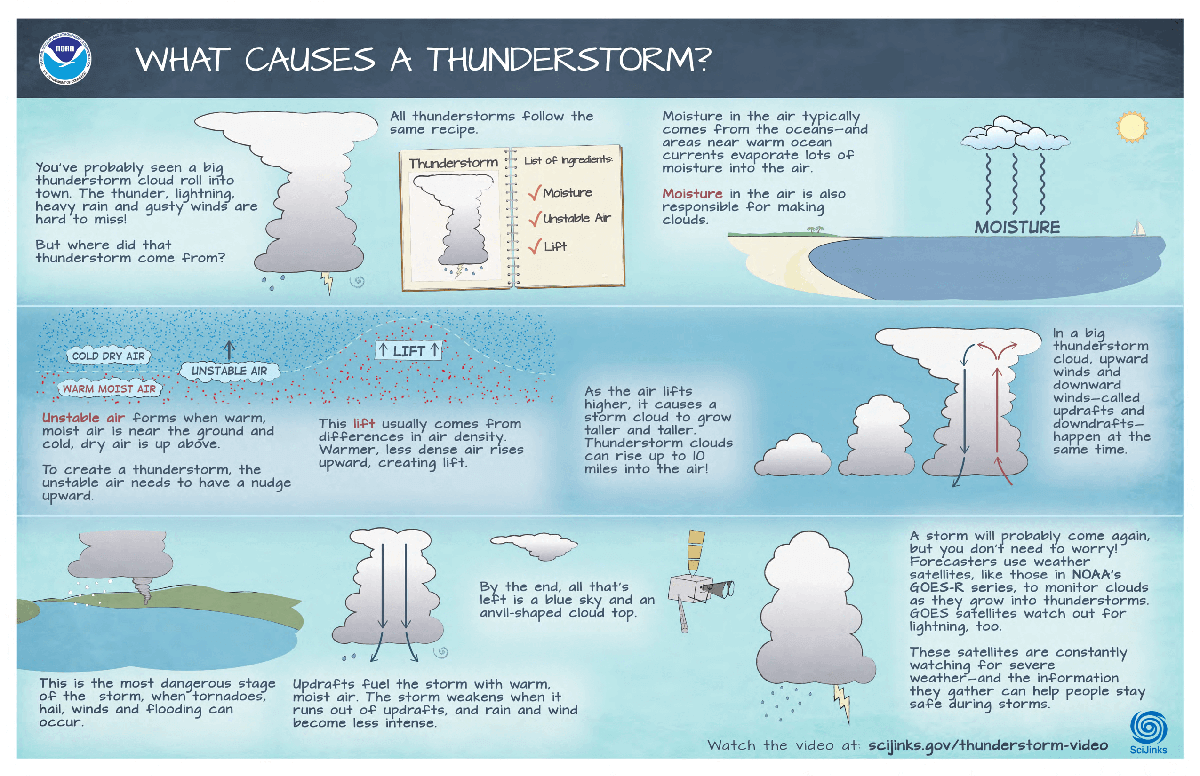
Video Link: https://scijinks.gov/thunderstorms-video/
Question 8.1.1
Summarize the three factors that create storms.
Question 8.1.2
Make at least 2 connections between thunderstorm formation and what you know about humidity.
Question 8.1.3
Describe a connection between formation of thunderstorms and what you know about transfer of energy.
Question 8.1.4
Think about how the Great Lakes system currently functions. What change in the Great Lakes system could impact this function, perhaps cause changes in frequency or strength of storms?
8.2. Text 2: Climate Change and Extreme Weather
Extreme weather gets a boost from climate change
Source: Environmental Defense Fund
Scientists are detecting a stronger link between the planet's warming and its changing weather patterns. Though it can be hard to pinpoint whether climate change intensified a particular weather event, the trajectory is clear — hotter heat waves, drier droughts, bigger storm surges and greater snowfall.
Storms and floods
As more evaporation leads to more moisture in the atmosphere, rainfall intensifies. For example, we now know that the rainfall from Hurricane Harvey was 15 percent more intense and three times as likely to occur due to human-induced climate change. We expect to see a higher frequency of Category 4 and 5 storms, also, as temperatures continue to rise.
While scientists aren't certain about whether climate change has led to more hurricanes, they are confident that rising sea levels are leading to higher storm surges and more floods.
Around half of sea-level rise since 1900 comes from the expansion of warming oceans, triggered by human-caused global warming. (Like all liquids, water generally expands as it heats up.) The rest of the rise comes from melting glaciers and ice sheets.
Snow and frigid weather
There is more moisture in a warmer atmosphere, which can lead to record snowfall.
It may seem counterintuitive, but the increase in snowfall during winter storms may be linked to climate change. Remember — there is more moisture in the warmer atmosphere. So when the temperatures are below freezing, snowfall can break records.
And scientists are studying a possible connection between a warming Arctic and cold spells in the eastern United States. The idea is that a rapidly warming Arctic can weaken the jet stream, allowing frigid polar air to travel farther south.
Question 8.2.1
Why are changes in storms, floods, and snowfall connected to rising temperatures?
Question 8.2.2
You may be familiar with the term, "polar vortex," which is associated with extremely cold temperatures that persist for a few days. Explain how this phenomenon is connected to climate change, based on what you read in the article.
8.3. Text 3: For the Midwest, Epic Flooding Is the Face of Climate Change
For the Midwest, Epic Flooding Is the Face of Climate Change (abridged)
By: MEGAN MOLTENI, 05.24.2019
Source: Wired.com
Scientists say it’s too early to tell to what degree this particularly relentless spring storm season is the result of human-induced climate change. But they agree that rising temperatures allow the atmosphere to hold more moisture—about 7 percent more for every 1 degree rise in Celsius—which produces more precipitation and has been fueling a pattern of more extreme weather events across the US. And perhaps more than any other part of the country, the Midwest has had its capacity to store excess water crippled by human developments like paved or concrete surfaces.
In 2015, researchers at the University of Iowa studied historical records of peak discharges from more than 700 stream gauge stations across the Midwest. Their analysis, reported in Nature, found that between 1962 and 2011, the magnitude of flood events hadn’t changed much. At a third of the locations, however, the number of floods was trending upward significantly.
More recent work, published in February by scientists at the University of Notre Dame, shows that floods aren't just getting more frequent—they'll also get more powerful in the future. Using a statistical method to blend data from global climate models with local information, the researchers predicted that the severity of extreme hydrologic events, so-called 100-year floods, hitting 20 watersheds in the Midwest and Great Lakes region will increase by as much as 30 percent by the end of the century. The approach, called “Hybrid Delta downscaling,” has been used to look at hydrological dynamics in other parts of the country before, but it was never applied to the Midwest. “What we’re seeing is that the past really is not a good predictor of the future,” says the study’s lead author, Kyuhyun Byun. “Especially when it comes to extreme weather events.”
In Byun’s case, the evidence is as much in his computer simulations as it is in his own waterlogged backyard. In South Bend, Indiana, where Notre Dame is located, the city is still recovering from back-to-back biblical deluges—a 500-year flood last spring preceded by a 1,000-year flood in 2016 that broke all historical records.
Besides all the damage to homes, businesses, and municipal infrastructure, increasingly frequent flooding events in the Midwest would have a huge impact on the nation’s ability to produce food. Wet fields make it difficult for farmers to operate their large, heavy planting machinery without getting stuck. And seedlings struggle to develop root systems when there’s too much moisture in the ground.
Question 8.3.1
This article attributes many of the changes in climate in the midwest to which factor?
Increase in moisture in the air
Decrease in temperature
Decrease in moisture in the air
Longer summer season
Decrease in temperature
Decrease in moisture in the air
Longer summer season
Question 8.3.2
Dr. Byun's research is discussed in this article. Given what you know of computer simulations, how do you think he uses them in his research?
8.4. Storms: Lake Effect Snow
Lake effect snow is a localized storm phenomena that results from a combination of variables.
When the lakes are not completely frozen over and the temperature of the lake is warmer than the temperature of the air, conditions are present that allows the air to increase the water vapor content. Air holds a certain amount of moisture dependent on its temperature. The amount of moisture in the air compared to the amount the air can hold is called relative humidity.
As wind currents move west to east (across the lake) and cold air moves down from Canada over the lakes, the air picks up moisture from the warmer lake and deposits it on the eastern or southeastern side (downwind) of the lake. This results in lake effect snow.
An increased rate of warming in the northern Great Lakes allow for more moisture to be absorbed. This may result in larger lake effect snow events to the east of a lake (see image).

Question 8.4.1
What does this text and image tell you about winter precipitation in the Great Lakes region?
Question 8.4.2
Explain how this text connects to the water cycle. What process is happening as the air moves over the warmer lake?
Question 8.4.3
Explain how this text connects to the humidity lab.
8.5. Trends in Great Lakes Storms
Connect the four texts to explain what is happening in the Great Lakes region.
Question 8.5.1
Why might thunderstorms around Chicago become more intense, distributing more rainfall on the area? Be sure to use evidence from at least 2 of the articles.
Question 8.5.2
Sometimes you hear people say that global warming is a "hoax" because it is cold or snowy. How would you respond to them to explain why a large snowstorm or persistent cold is occurring?
Question 8.5.3
If you could work on a research team, like the ones that provided the information in the articles, what question would you want to investigate to learn more about this? Do you have ideas for what resources or tools you would use?
8.6. Revise GL Sage Modeler
In the Sage Modeler file below, use what you have learned to connect variables to storm strength.
Refer to Sage Modeler Guide for help drawing arrows, setting relationships, and labeling.
Question 8.6.1
Add a screenshot of your model with humidity added.
Screenshot:
To take a screenshot:
Step 1: Hold down the Ctrl and Shift keys at once, then press the Switch window button.
Step 2: Chrome’s cursor will be temporarily replaced with a crosshair. Click and drag a square across the portion of the screen you want to save, then release the trackpad or mouse button.
The partial screenshot will be saved in the Downloads folder, the same as a full screenshot.
Upload files that are less than 5MB in size.
| File | Delete |
|---|---|
Upload files to the space allocated by your teacher.
Question 8.6.2
Explain what you connected on the sage modeler above. Why did you choose to connect those specific variables?
Question 8.6.3
Explain using the connections on Sage Modeler how increasing global temperature leads to stronger thunderstorms or an increase in winter precipitation. Discuss what you read in the prior pages and refer to specific parts of sage modeler that connect.
Lesson 9 Overview
In this lesson, students use a "data snapshot" model to look at temperature and precipitation data since 2000. This is a great lesson to discuss features of maps, especially the color scale and what the different units mean. In the temperature maps, students are comparing current data each year to a prior 30 year average represented as 0. In the precipitation maps, students are comparing current data each year to a prior 30 year average represented as 100%.
In the model there are sensors on 5 major cities in the Great Lakes, Chicago, Detroit, Milwaukee, Cleveland and Buffalo. The data is recorded in CODAP and students can use the graphing feature to see how the amount changes in different cities over a number of years.
In the next lesson they look at the long term changes, so this lesson really focuses on understanding how to read the maps, what information they are getting from the maps, and looking over time at a particular city or month to see if they can determine any trends.
Credits
Climate.gov data snapshot
Lesson 9 Activities
- 9.1. Data Snapshot Tool
9.0. Student Directions and Resources
We will analyze what the past 20 years have looked like in the Great Lakes. To do this we will use a simulation that uses Climate.gov data. You will be looking at 4 different months (1 per season) over the past 18-19 years.
We want to see if what has happened since 2000 tells us anything about future temperature and precipitation projections. We also want to see how these changes look seasonally. You will collect and record data, then we will have a class discussion to think about what this data means.
9.1. Data Snapshot Tool
Use the simulation below to collect data. Collect data for temperature or precipitation by changing the months or years and clicking "record data" before you move to the next month/year. Use the graphing feature to visualize your data, by dragging from the table the variable you want on the x or y axis.
Notes on using the simulation:
- Make sure "auto update" is clicked (dark blue), so the map will update.
- Wait a few seconds after changing month or year for the map to update (you will see the new map show up).
- Change the months or years to see look for patterns in the data.
- Look at temperature or precipitation maps.
Question 9.1.1
Choose a month and look at it over a few different years. What do you notice about the temperature change from the 30 year average (represented as 0)?
Question 9.1.2
Choose a month and look at it over a few different years. What do you notice about the precipitation change from the 30 year average (represented as 100%)?
Question 9.1.3
Do certain cities have more temperature change than others? Explain using at least 5 pieces of evidence.
Question 9.1.4
Do certain cities have more precipitation change than others? Explain using at least 5 pieces of evidence.
Lesson 10 Overview
In this lesson, students have graphs that show the compiled data from the data snapshot model in lesson 9. Students compare these to the conclusions they developed using the model. They also use this data to think about the differences by season.
In addition to the data snapshots graphs, there are graphs from GLISA that look at water temperature and lake level trends. They also use this lesson to see the impact of rising temperature on ice cover on the lakes.
Credits
ice cover graph: https://www.glerl.noaa.gov/data/ice/imgs/IceCover_avg_1973_2020.png
Lesson 10 Activities
- 10.1. Changes in Temperature by Season
- 10.2. Precipitation Differences by Season
- 10.3. Trends in the Great Lakes
- 10.4. Lake Temperature and Lake Levels
- 10.5. Ice Cover in the Great Lakes
10.0. Student Directions and Resources
The model in the previous lesson allowed you to determine some trends, perhaps in a single city or a single time of year. But, maybe you were frustrated by not being able to see the whole picture. Climate scientists often have to go through a lot of data to determine trends. In this lesson, you will see graphs that have used the data from the model in the previous lesson. There will also be data from other scientific organizations in the Great Lakes, like University of Michigan's Great Lakes Integrated Sciences and Assessments (GLISA).
10.1. Changes in Temperature by Season
| Season (2000-2018) | Spring | Summer | Winter | Fall |
| Average Temp Anomaly (degrees F) | 0.54 | 0.54 | 1.15 | 0.53 |

Question 10.1.1
This graph represents temperature anomaly, which is the difference from an established average (here each year's temp is compared to the average from 1970-1999). Where do the majority of the data fall?
Above 0
Below 0
Below 0
Question 10.1.2
Which season is increasing in temperature the most?
Spring
Summer
Winter
Fall
Summer
Winter
Fall
Question 10.1.3
What is something you notice on this graph? Provide specific evidence to support your observation.
10.2. Precipitation Differences by Season
| Season (2000-2018) | Spring | Summer | Winter | Fall |
| % Average Annual Precipitation | 102.5 | 98.3 | 103.4 | 94.2 |

Question 10.2.1
Which number is equal to the average annual precipitation?
0%
60%
100%
180%
60%
100%
180%
Question 10.2.2
In which seasons are the increases in precipitation the greatest? Use at least 3 pieces of evidence from the graph and table.
Question 10.2.3
What is something you notice on this graph? Provide specific evidence to support your observation.
10.3. Trends in the Great Lakes
A warmer atmosphere holds more moisture, increasing the frequency and intensity of heavy rain and snow events. Overall U.S. annual precipitation increased 4% between 1901 and 2015, but the Great Lakes region saw an almost 10% increase over this interval with more of this precipitation coming as unusually large events. In the future, precipitation will likely redistribute across the seasons. We expect wetter winters and springs, while summer precipitation should decrease by 5-15% for most of Great Lake states by 2100.
(source: http://elpc.org/wp-content/uploads/2019/03/Great-Lakes-Climate-Change-Report.pdf)
The text above is from the Climate Change Report from the Environmental Law and Policy Center. Use the text along with the graphs on page 1 and 2 to answer the following questions.
Graphs from page 1 and 2:
Question 10.3.1
Explain what evidence the graphs on pages 1 and 2 provide to support or refute this statement in the Climate Change report. Use specific data from those graphs.
Question 10.3.2
Based on what you've learned, why do you think precipitation may decrease in the summer?
Question 10.3.3
Which of the factors in the Great Lakes may be impacted by these changes? How will they be impacted or change?
10.4. Lake Temperature and Lake Levels
In the 2019 Climate Trends report from GLISA, there is additional focus on lake water temperature and lake water levels. The following graphs show changes from 1950-2019 in the 5 lakes (Michigan and Huron are grouped together).

Retrieved from: (https://glisa.umich.edu/2019-annual-climate-trends-and-impacts-summary-for-the-great-lakes-basin/)
Question 10.4.1
What does the data indicate is happening to lake water temperature over time? Provide specific evidence from the graphs.
Question 10.4.2
If you were going to compare lake water temperature to another set of graphs, which one would you choose? Do you think it might be connected? Why?
Question 10.4.3
Lake water levels are another incredibly important factor. What do the graphs indicate is currently happening to lake levels? Is there a trend over time?
Question 10.4.4
If you were going to compare lake water levels to another set of graphs, which one would you choose? Do you think it might be connected? Why?
Question 10.4.5
Ice cover (when the lakes freeze over) is another indicator that is being used when looking at the Great Lakes system. Based on the data you've seen, predict what is happening with ice cover in the Great Lakes (increasing, decreasing or staying the same) and explain your reasoning for your prediction.
10.5. Ice Cover in the Great Lakes
Ice cover is another indicator and major factor that affects the Great Lakes' seasonal weather patterns. Ice cover is impacted by a number of different factors, and is especially dependent on the location of the jet stream, a band of fast moving air in the atmosphere.
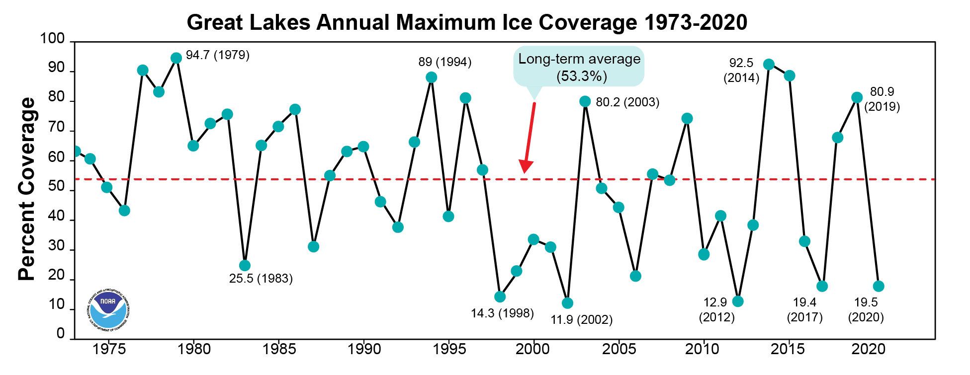
Question 10.5.1
Count the number of data points above the long term average between 1980 and 2000, and the number above the long term average between 2000-2020. What do you notice?
Question 10.5.2
From 1975-2020, in which years are the 5 lowest amount of ice cover?
Question 10.5.3
Your friend tells you that he heard that the ice cover this year is really high. In fact, he heard on the news that it is the highest in 10 years. Given the data you see on the chart, what do you think? Why do you think ice cover is high? Do you think it will continue to stay high in the years following?
Question 10.5.4
What connection(s) can you make about temperature and precipitation trends you noticed in the maps and the data snapshot model? How might these impact ice cover in the Great Lakes?
Lesson 11 Overview
In this lesson, students develop a final model to explain how rising global temperatures and key features in the Great Lakes system will result in rising precipitation. They will modify a final sage modeler file and use the simulate and graphing functions to provide evidence of connections that aren't directly connected by an arrow.
Lesson 11 Activities
- 11.1. Factors of Great Lakes Climate
11.0. Student Directions and Resources
You have learned a LOT about the factors influencing climate in the Great Lakes. You are going to put that together to develop your final model.
11.1. Factors of Great Lakes Climate
In the Sage Modeler window below, you have the model we have added to throughout this unit. Use this model to develop a final explanation for the unit, including collecting evidence by using the simulate and graphing functions.
Question 11.1.1
Provide an overall explanation of the parts of the model. Include what you have learned to explain the connections between specific variables.
Question 11.1.2
1. Make a connection between two variables that aren’t connected by an arrow, to explain a concept you learned about (If you wish to add a new variable, you may but make sure you connect it to existing ones).
2. Use the simulate and graphing functions to provide evidence that support what the connection is. Describe the trend on the graph for your evidence.
3. Support the connection you made with science content (reading, understanding from a lesson, lab, etc.).
Question 11.1.3
1. Make a 2nd connection between two variables that aren’t connected by an arrow to explain a concept you learned about (If you wish to add a new variable, you may but make sure you connect it to existing ones).
2. Use the simulate and graphing functions to provide evidence that support what the connection is. Describe the trend on the graph for your evidence.
3. Support the connection you made with science content (reading, understanding from a lesson, lab, etc.).